Friday, 12 April 2019

R - Chi Square Test

Chi-Square test is a statistical method to determine if two categorical variables have a significant correlation between them. Both those variables should be from same population and they should be categorical like − Yes/No, Male/Female, Red/Green etc.
For example, we can build a data set with observations on people's ice-cream buying pattern and try to correlate the gender of a person with the flavor of the ice-cream they prefer. If a correlation is found we can plan for appropriate stock of flavors by knowing the number of gender of people visiting.

Syntax

The function used for performing chi-Square test is chisq.test().
The basic syntax for creating a chi-square test in R is −
chisq.test(data)
Following is the description of the parameters used −
  • data is the data in form of a table containing the count value of the variables in the observation.

Example

We will take the Cars93 data in the "MASS" library which represents the sales of different models of car in the year 1993.
 Live Demo
library("MASS")
print(str(Cars93))
When we execute the above code, it produces the following result −
'data.frame':   93 obs. of  27 variables: 
 $ Manufacturer      : Factor w/ 32 levels "Acura","Audi",..: 1 1 2 2 3 4 4 4 4 5 ... 
 $ Model             : Factor w/ 93 levels "100","190E","240",..: 49 56 9 1 6 24 54 74 73 35 ... 
 $ Type              : Factor w/ 6 levels "Compact","Large",..: 4 3 1 3 3 3 2 2 3 2 ... 
 $ Min.Price         : num  12.9 29.2 25.9 30.8 23.7 14.2 19.9 22.6 26.3 33 ... 
 $ Price             : num  15.9 33.9 29.1 37.7 30 15.7 20.8 23.7 26.3 34.7 ... 
 $ Max.Price         : num  18.8 38.7 32.3 44.6 36.2 17.3 21.7 24.9 26.3 36.3 ... 
 $ MPG.city          : int  25 18 20 19 22 22 19 16 19 16 ... 
 $ MPG.highway       : int  31 25 26 26 30 31 28 25 27 25 ... 
 $ AirBags           : Factor w/ 3 levels "Driver & Passenger",..: 3 1 2 1 2 2 2 2 2 2 ... 
 $ DriveTrain        : Factor w/ 3 levels "4WD","Front",..: 2 2 2 2 3 2 2 3 2 2 ... 
 $ Cylinders         : Factor w/ 6 levels "3","4","5","6",..: 2 4 4 4 2 2 4 4 4 5 ... 
 $ EngineSize        : num  1.8 3.2 2.8 2.8 3.5 2.2 3.8 5.7 3.8 4.9 ... 
 $ Horsepower        : int  140 200 172 172 208 110 170 180 170 200 ... 
 $ RPM               : int  6300 5500 5500 5500 5700 5200 4800 4000 4800 4100 ... 
 $ Rev.per.mile      : int  2890 2335 2280 2535 2545 2565 1570 1320 1690 1510 ... 
 $ Man.trans.avail   : Factor w/ 2 levels "No","Yes": 2 2 2 2 2 1 1 1 1 1 ... 
 $ Fuel.tank.capacity: num  13.2 18 16.9 21.1 21.1 16.4 18 23 18.8 18 ... 
 $ Passengers        : int  5 5 5 6 4 6 6 6 5 6 ... 
 $ Length            : int  177 195 180 193 186 189 200 216 198 206 ... 
 $ Wheelbase         : int  102 115 102 106 109 105 111 116 108 114 ... 
 $ Width             : int  68 71 67 70 69 69 74 78 73 73 ... 
 $ Turn.circle       : int  37 38 37 37 39 41 42 45 41 43 ... 
 $ Rear.seat.room    : num  26.5 30 28 31 27 28 30.5 30.5 26.5 35 ... 
 $ Luggage.room      : int  11 15 14 17 13 16 17 21 14 18 ... 
 $ Weight            : int  2705 3560 3375 3405 3640 2880 3470 4105 3495 3620 ... 
 $ Origin            : Factor w/ 2 levels "USA","non-USA": 2 2 2 2 2 1 1 1 1 1 ... 
 $ Make              : Factor w/ 93 levels "Acura Integra",..: 1 2 4 3 5 6 7 9 8 10 ... 
The above result shows the dataset has many Factor variables which can be considered as categorical variables. For our model we will consider the variables "AirBags" and "Type". Here we aim to find out any significant correlation between the types of car sold and the type of Air bags it has. If correlation is observed we can estimate which types of cars can sell better with what types of air bags.
 Live Demo
# Load the library.
library("MASS")

# Create a data frame from the main data set.
car.data <- data.frame(Cars93$AirBags, Cars93$Type)

# Create a table with the needed variables.
car.data = table(Cars93$AirBags, Cars93$Type) 
print(car.data)

# Perform the Chi-Square test.
print(chisq.test(car.data))
When we execute the above code, it produces the following result −
                     Compact Large Midsize Small Sporty Van
  Driver & Passenger       2     4       7     0      3   0
  Driver only              9     7      11     5      8   3
  None                     5     0       4    16      3   6

         Pearson's Chi-squared test

data:  car.data
X-squared = 33.001, df = 10, p-value = 0.0002723

Warning message:
In chisq.test(car.data) : Chi-squared approximation may be incorrect

Conclusion

The result shows the p-value of less than 0.05 which indicates a string correlation.
R - Survival Analysis

Survival analysis deals with predicting the time when a specific event is going to occur. It is also known as failure time analysis or analysis of time to death. For example predicting the number of days a person with cancer will survive or predicting the time when a mechanical system is going to fail.
The R package named survival is used to carry out survival analysis. This package contains the function Surv() which takes the input data as a R formula and creates a survival object among the chosen variables for analysis. Then we use the function survfit() to create a plot for the analysis.

Install Package

install.packages("survival")

Syntax

The basic syntax for creating survival analysis in R is −
Surv(time,event)
survfit(formula)
Following is the description of the parameters used −
  • time is the follow up time until the event occurs.
  • event indicates the status of occurrence of the expected event.
  • formula is the relationship between the predictor variables.

Example

We will consider the data set named "pbc" present in the survival packages installed above. It describes the survival data points about people affected with primary biliary cirrhosis (PBC) of the liver. Among the many columns present in the data set we are primarily concerned with the fields "time" and "status". Time represents the number of days between registration of the patient and earlier of the event between the patient receiving a liver transplant or death of the patient.
# Load the library.
library("survival")

# Print first few rows.
print(head(pbc))
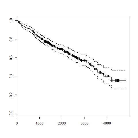
When we execute the above code, it produces the following result and chart −
  id time status trt      age sex ascites hepato spiders edema bili chol
1  1  400      2   1 58.76523   f       1      1       1   1.0 14.5  261
2  2 4500      0   1 56.44627   f       0      1       1   0.0  1.1  302
3  3 1012      2   1 70.07255   m       0      0       0   0.5  1.4  176
4  4 1925      2   1 54.74059   f       0      1       1   0.5  1.8  244
5  5 1504      1   2 38.10541   f       0      1       1   0.0  3.4  279
6  6 2503      2   2 66.25873   f       0      1       0   0.0  0.8  248
  albumin copper alk.phos    ast trig platelet protime stage
1    2.60    156   1718.0 137.95  172      190    12.2     4
2    4.14     54   7394.8 113.52   88      221    10.6     3
3    3.48    210    516.0  96.10   55      151    12.0     4
4    2.54     64   6121.8  60.63   92      183    10.3     4
5    3.53    143    671.0 113.15   72      136    10.9     3
6    3.98     50    944.0  93.00   63       NA    11.0     3
From the above data we are considering time and status for our analysis.

Applying Surv() and survfit() Function

Now we proceed to apply the Surv() function to the above data set and create a plot that will show the trend.
# Load the library.
library("survival")

# Create the survival object. 
survfit(Surv(pbc$time,pbc$status == 2)~1)

# Give the chart file a name.
png(file = "survival.png")

# Plot the graph. 
plot(survfit(Surv(pbc$time,pbc$status == 2)~1))

# Save the file.
dev.off()
When we execute the above code, it produces the following result and chart −
Call: survfit(formula = Surv(pbc$time, pbc$status == 2) ~ 1)

      n  events  median 0.95LCL 0.95UCL 
    418     161    3395    3090    3853 
Survival Analysis Using R
The trend in the above graph helps us predicting the probability of survival at the end of a certain number of days.

R - Random Forest

In the random forest approach, a large number of decision trees are created. Every observation is fed into every decision tree. The most common outcome for each observation is used as the final output. A new observation is fed into all the trees and taking a majority vote for each classification model.
An error estimate is made for the cases which were not used while building the tree. That is called an OOB (Out-of-bag) error estimate which is mentioned as a percentage.
The R package "randomForest" is used to create random forests.

Install R Package

Use the below command in R console to install the package. You also have to install the dependent packages if any.
install.packages("randomForest)
The package "randomForest" has the function randomForest() which is used to create and analyze random forests.

Syntax

The basic syntax for creating a random forest in R is −
randomForest(formula, data)
Following is the description of the parameters used −
  • formula is a formula describing the predictor and response variables.
  • data is the name of the data set used.

Input Data

We will use the R in-built data set named readingSkills to create a decision tree. It describes the score of someone's readingSkills if we know the variables "age","shoesize","score" and whether the person is a native speaker.
Here is the sample data.
# Load the party package. It will automatically load other
# required packages.
library(party)

# Print some records from data set readingSkills.
print(head(readingSkills))
When we execute the above code, it produces the following result and chart −
  nativeSpeaker   age   shoeSize      score
1           yes     5   24.83189   32.29385
2           yes     6   25.95238   36.63105
3            no    11   30.42170   49.60593
4           yes     7   28.66450   40.28456
5           yes    11   31.88207   55.46085
6           yes    10   30.07843   52.83124
Loading required package: methods
Loading required package: grid
...............................
...............................

Example

We will use the randomForest() function to create the decision tree and see it's graph.
# Load the party package. It will automatically load other
# required packages.
library(party)
library(randomForest)

# Create the forest.
output.forest <- randomForest(nativeSpeaker ~ age + shoeSize + score, 
           data = readingSkills)

# View the forest results.
print(output.forest) 

# Importance of each predictor.
print(importance(fit,type = 2)) 
When we execute the above code, it produces the following result −
Call:
 randomForest(formula = nativeSpeaker ~ age + shoeSize + score,     
                 data = readingSkills)
               Type of random forest: classification
                     Number of trees: 500
No. of variables tried at each split: 1

        OOB estimate of  error rate: 1%
Confusion matrix:
    no yes class.error
no  99   1        0.01
yes  1  99        0.01
         MeanDecreaseGini
age              13.95406
shoeSize         18.91006
score            56.73051

Conclusion

From the random forest shown above we can conclude that the shoesize and score are the important factors deciding if someone is a native speaker or not. Also the model has only 1% error which means we can predict with 99% accuracy.

R - Decision Tree

Decision tree is a graph to represent choices and their results in form of a tree. The nodes in the graph represent an event or choice and the edges of the graph represent the decision rules or conditions. It is mostly used in Machine Learning and Data Mining applications using R.
Examples of use of decision tress is − predicting an email as spam or not spam, predicting of a tumor is cancerous or predicting a loan as a good or bad credit risk based on the factors in each of these. Generally, a model is created with observed data also called training data. Then a set of validation data is used to verify and improve the model. R has packages which are used to create and visualize decision trees. For new set of predictor variable, we use this model to arrive at a decision on the category (yes/No, spam/not spam) of the data.
The R package "party" is used to create decision trees.

Install R Package

Use the below command in R console to install the package. You also have to install the dependent packages if any.
install.packages("party")
The package "party" has the function ctree() which is used to create and analyze decison tree.

Syntax

The basic syntax for creating a decision tree in R is −
ctree(formula, data)
Following is the description of the parameters used −
  • formula is a formula describing the predictor and response variables.
  • data is the name of the data set used.

Input Data

We will use the R in-built data set named readingSkills to create a decision tree. It describes the score of someone's readingSkills if we know the variables "age","shoesize","score" and whether the person is a native speaker or not.
Here is the sample data.
# Load the party package. It will automatically load other
# dependent packages.
library(party)

# Print some records from data set readingSkills.
print(head(readingSkills))
When we execute the above code, it produces the following result and chart −
  nativeSpeaker   age   shoeSize      score
1           yes     5   24.83189   32.29385
2           yes     6   25.95238   36.63105
3            no    11   30.42170   49.60593
4           yes     7   28.66450   40.28456
5           yes    11   31.88207   55.46085
6           yes    10   30.07843   52.83124
Loading required package: methods
Loading required package: grid
...............................
...............................

Example

We will use the ctree() function to create the decision tree and see its graph.
# Load the party package. It will automatically load other
# dependent packages.
library(party)

# Create the input data frame.
input.dat <- readingSkills[c(1:105),]

# Give the chart file a name.
png(file = "decision_tree.png")

# Create the tree.
  output.tree <- ctree(
  nativeSpeaker ~ age + shoeSize + score, 
  data = input.dat)

# Plot the tree.
plot(output.tree)

# Save the file.
dev.off()
When we execute the above code, it produces the following result −
null device 
          1 
Loading required package: methods
Loading required package: grid
Loading required package: mvtnorm
Loading required package: modeltools
Loading required package: stats4
Loading required package: strucchange
Loading required package: zoo

Attaching package: ‘zoo’

The following objects are masked from ‘package:base’:

   as.Date, as.Date.numeric

Loading required package: sandwich
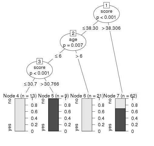
Decision Tree using R

Conclusion

From the decision tree shown above we can conclude that anyone whose readingSkills score is less than 38.3 and age is more than 6 is not a native Speaker.

R - Nonlinear Least Square

When modeling real world data for regression analysis, we observe that it is rarely the case that the equation of the model is a linear equation giving a linear graph. Most of the time, the equation of the model of real world data involves mathematical functions of higher degree like an exponent of 3 or a sin function. In such a scenario, the plot of the model gives a curve rather than a line. The goal of both linear and non-linear regression is to adjust the values of the model's parameters to find the line or curve that comes closest to your data. On finding these values we will be able to estimate the response variable with good accuracy.
In Least Square regression, we establish a regression model in which the sum of the squares of the vertical distances of different points from the regression curve is minimized. We generally start with a defined model and assume some values for the coefficients. We then apply the nls() function of R to get the more accurate values along with the confidence intervals.

Syntax

The basic syntax for creating a nonlinear least square test in R is −
nls(formula, data, start)
Following is the description of the parameters used −
  • formula is a nonlinear model formula including variables and parameters.
  • data is a data frame used to evaluate the variables in the formula.
  • start is a named list or named numeric vector of starting estimates.

Example

We will consider a nonlinear model with assumption of initial values of its coefficients. Next we will see what is the confidence intervals of these assumed values so that we can judge how well these values fir into the model.
So let's consider the below equation for this purpose −
a = b1*x^2+b2
Let's assume the initial coefficients to be 1 and 3 and fit these values into nls() function.
 Live Demo
xvalues <- c(1.6,2.1,2,2.23,3.71,3.25,3.4,3.86,1.19,2.21)
yvalues <- c(5.19,7.43,6.94,8.11,18.75,14.88,16.06,19.12,3.21,7.58)

# Give the chart file a name.
png(file = "nls.png")


# Plot these values.
plot(xvalues,yvalues)


# Take the assumed values and fit into the model.
model <- nls(yvalues ~ b1*xvalues^2+b2,start = list(b1 = 1,b2 = 3))

# Plot the chart with new data by fitting it to a prediction from 100 data points.
new.data <- data.frame(xvalues = seq(min(xvalues),max(xvalues),len = 100))
lines(new.data$xvalues,predict(model,newdata = new.data))

# Save the file.
dev.off()

# Get the sum of the squared residuals.
print(sum(resid(model)^2))

# Get the confidence intervals on the chosen values of the coefficients.
print(confint(model))
When we execute the above code, it produces the following result −
[1] 1.081935
Waiting for profiling to be done...
       2.5%    97.5%
b1 1.137708 1.253135
b2 1.497364 2.496484
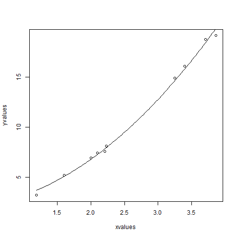
Non Linear least square R
We can conclude that the value of b1 is more close to 1 while the value of b2 is more close to 2 and not 3.

R - Time Series Analysis

Time series is a series of data points in which each data point is associated with a timestamp. A simple example is the price of a stock in the stock market at different points of time on a given day. Another example is the amount of rainfall in a region at different months of the year. R language uses many functions to create, manipulate and plot the time series data. The data for the time series is stored in an R object called time-series object. It is also a R data object like a vector or data frame.
The time series object is created by using the ts() function.

Syntax

The basic syntax for ts() function in time series analysis is −
timeseries.object.name <-  ts(data, start, end, frequency)
Following is the description of the parameters used −
  • data is a vector or matrix containing the values used in the time series.
  • start specifies the start time for the first observation in time series.
  • end specifies the end time for the last observation in time series.
  • frequency specifies the number of observations per unit time.
Except the parameter "data" all other parameters are optional.

Example

Consider the annual rainfall details at a place starting from January 2012. We create an R time series object for a period of 12 months and plot it.
 Live Demo
# Get the data points in form of a R vector.
rainfall <- c(799,1174.8,865.1,1334.6,635.4,918.5,685.5,998.6,784.2,985,882.8,1071)

# Convert it to a time series object.
rainfall.timeseries <- ts(rainfall,start = c(2012,1),frequency = 12)

# Print the timeseries data.
print(rainfall.timeseries)

# Give the chart file a name.
png(file = "rainfall.png")

# Plot a graph of the time series.
plot(rainfall.timeseries)

# Save the file.
dev.off()
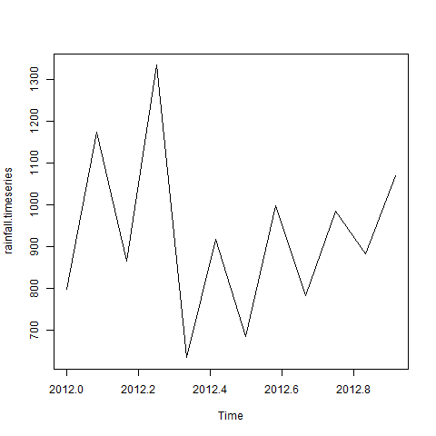
When we execute the above code, it produces the following result and chart −
Jan    Feb    Mar    Apr    May     Jun    Jul    Aug    Sep
2012  799.0  1174.8  865.1  1334.6  635.4  918.5  685.5  998.6  784.2
        Oct    Nov    Dec
2012  985.0  882.8 1071.0
The Time series chart −
Time Series using R

Different Time Intervals

The value of the frequency parameter in the ts() function decides the time intervals at which the data points are measured. A value of 12 indicates that the time series is for 12 months. Other values and its meaning is as below −
  • frequency = 12 pegs the data points for every month of a year.
  • frequency = 4 pegs the data points for every quarter of a year.
  • frequency = 6 pegs the data points for every 10 minutes of an hour.
  • frequency = 24*6 pegs the data points for every 10 minutes of a day.

Multiple Time Series

We can plot multiple time series in one chart by combining both the series into a matrix.
 Live Demo
# Get the data points in form of a R vector.
rainfall1 <- c(799,1174.8,865.1,1334.6,635.4,918.5,685.5,998.6,784.2,985,882.8,1071)
rainfall2 <- 
           c(655,1306.9,1323.4,1172.2,562.2,824,822.4,1265.5,799.6,1105.6,1106.7,1337.8)

# Convert them to a matrix.
combined.rainfall <-  matrix(c(rainfall1,rainfall2),nrow = 12)

# Convert it to a time series object.
rainfall.timeseries <- ts(combined.rainfall,start = c(2012,1),frequency = 12)

# Print the timeseries data.
print(rainfall.timeseries)

# Give the chart file a name.
png(file = "rainfall_combined.png")

# Plot a graph of the time series.
plot(rainfall.timeseries, main = "Multiple Time Series")

# Save the file.
dev.off()
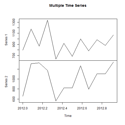
When we execute the above code, it produces the following result and chart −
           Series 1  Series 2
Jan 2012    799.0    655.0
Feb 2012   1174.8   1306.9
Mar 2012    865.1   1323.4
Apr 2012   1334.6   1172.2
May 2012    635.4    562.2
Jun 2012    918.5    824.0
Jul 2012    685.5    822.4
Aug 2012    998.6   1265.5
Sep 2012    784.2    799.6
Oct 2012    985.0   1105.6
Nov 2012    882.8   1106.7
Dec 2012   1071.0   1337.8
The Multiple Time series chart −
Combined Time series is using R