Introduction:
Learn how the SHAP library works under the hood
SHAP library in Python
In this article, we will study the different methods that can be used to calculate the SHAP values, and each method will be implemented in Python from scratch. However, the code is only used to show how the algorithms work, and it is not efficient for real-world applications. The SHAP library in Python can be used to calculate the SHAP values of a model efficiently, and in this article, we will show you briefly how to use this library. We also use it to validate the output of the Python scripts given in each section (the code has been tested with shap 0.40.0).
Explaining the predictions of a model
Most machine learning models are designed to predict a target. Here the accuracy of the prediction is very important, however, we also need to understand why a model makes a certain prediction. So, we need a tool to explain a model. By explaining, we mean that we want to have a qualitative understanding of the relationship between the prediction of the model and the components of the data instance that the model used to generate that prediction. These components can be a feature of the data instance (if we have a tabular data set) or a set of pixels in an image or a word in a text document. We want to see how the presence (or absence) of these components affect the prediction.
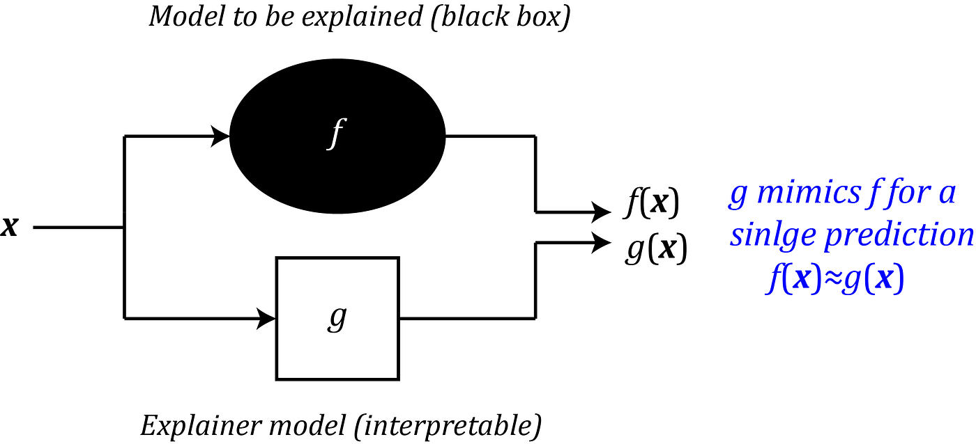
Some models in machine learning like linear regression or decision trees are interpretable. Here interpretability refers to how easy it is for humans to understand the processes the model uses to make a prediction. For example, if we plot a decision tree classifier, we can easily understand how it makes a certain prediction. On the other hand, deep learning models are like a black box, and we cannot easily understand how these modes make a prediction. SHAP is an individualized model-agnostic explainer. A model-agnostic method assumes that the model to be explained is a black box and doesn’t know how the model internally works. So the model-agnostic method can only access the input data and the prediction of the model to be explained. An individualized model-agnostic explainer is an interpretable model itself. The explainer can approximately make the same prediction of the model to be explained for a specific data instance (Figure 1). Now we can assume that this interpretable model is mimicking the process that the original model uses to make that single specific prediction. Hence, we say that the interpretable model can explain the original model. In summary, SHAP can explain any machine learning model without knowing how that model internally works, and it can achieve this using the concepts of game theory. So to understand it, first, we need to get familiar with the Shapley values.
Shapley values
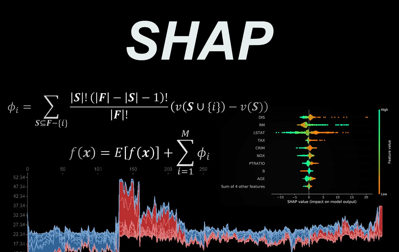
The Shapley value is a mathematical concept in game theory that was introduced by Lloyd Shapley in 1951. He was later awarded the Nobel Prize in Economics for this work. Suppose that we have a cooperative game with M players numbered from 1 to M, and let F denote the set of players, so F = {1, 2, . . . , M}. A coalition, S, is defined to be a subset of F (S ⊆ F), and we also assume that the empty set, ∅, is a coalition that has no players. For example, if we have 3 players, then the possible coalitions are:

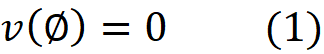
The set F is also a coalition, and we call it the grand coalition. It can be easily shown that for M players, we have 2M coalitions. Now we define a function v that maps each coalition to a real number. v is called a characteristic function. So, for each coalition S, the quantity v(S) is a real number and is called the worth of the coalition S. It is considered as the total gain or collective payoff that the players in that coalition can obtain if they act together. Since the empty coalition has no players, we can assume that
Now we want to know that in a coalitional game with M players, what is the contribution of each player to the total payoff? In other words, what is the fairest way to divide the total gain among the players?
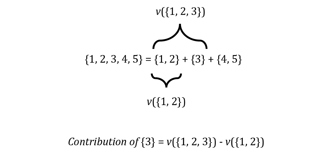
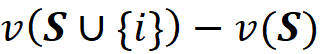
We can show you how to solve this problem using an example. Imagine that we have a game with 5 players, so F = {1, 2, . . . , 5}. Suppose we form the grand coalition F by adding the players to an empty set one at a time, so each time that we add a new player, we form a new coalition of F. For example, we first add {1} to the empty set, so the current set of players is {1} which is a coalition of F. Then we add {2} and the current set is the coalition {1,2} and we continue until we get F={1, 2, 3, 4, 5}. As each player is added to the current set of players, he increases the total gain of the previous coalition. For example when the current set is {1, 2}, the total gain v({1, 2}). After adding {3}, the total gain becomes v({1, 2, 3}). Now we can assume that the contribution of {3} to the current coalition is the difference between the value of the current coalition (including {3}) and the previous coalition which didn’t include {3}:
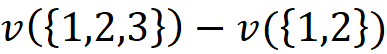
After adding {3}, we can ad {4} and {5} and they will also change the total gain. However, it doesn’t affect the contribution of {3}, so the previous equation still gives the contribution of {3} (Figure 2). However, there is a problem here. The order of the addition of players is also important.
Suppose that these players are the employees of a department in a company. The company first hires {1}. Then they figure out that they lack a skill set, so they hire {2}. After hiring {2} the total gain of the company is increased by $10000, and this is the contribution of {2} when added to {1}. After hiring {3}, the contribution of {3} is just $2000. In addition, suppose that the employees {2} and {3} have similar skill sets. Now employee {3} can claim that if he had been hired sooner, he would have the same contribution of {2}. In other words, the contribution of {3} when added to {1} could be also $10000. So, to have a fair evaluation of the contribution of each player, we should also need to take into account the order in which they are added to form the grand coalition.
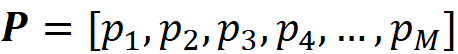
In fact, to have a fair evaluation of the contribution of the player {i}, we should form all the permutations of F and calculate the contribution of {i} in each of them and then take the average of these contributions. For example, one possible permutation of F={1, 2, 3, 4, 5} is:
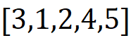
And the contribution of {3} in this permutation is:
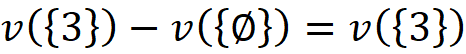
Another permutation can be:
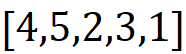
And the contribution of {3} in this permutation is:

It is important to note that the characteristic function v, takes a coalition as its argument, not a permutation. A coalition is a set, so the order of elements in that is not important, but a permutation is an ordered collection of elements. In a permutation like [3,1,2,4,5], 3 is the first player and 5 is the last player added to the team. So, for each permutation, the order of elements can change their contribution to the total gain, however, the total gain or the worth of the permutation only depends on the elements, not their order. So:

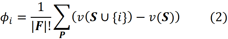
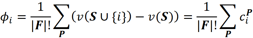
So, for each permutation P, we need to first calculate the worth of the coalition of the players which were added before {i}. Let’s call this coalition S. Then we need to calculate the worth of the coalition which is formed by adding {i} to S, and we call this coalition S U {i}. Now the contribution of the player {i} denoted by ϕᵢ is:
The total number of permutations of the grand coalition F is |F|! (here |F| means the number of elements of set F), so we divide the sum of the contributions by that to take the average of contributions for {i} (Figure 3).
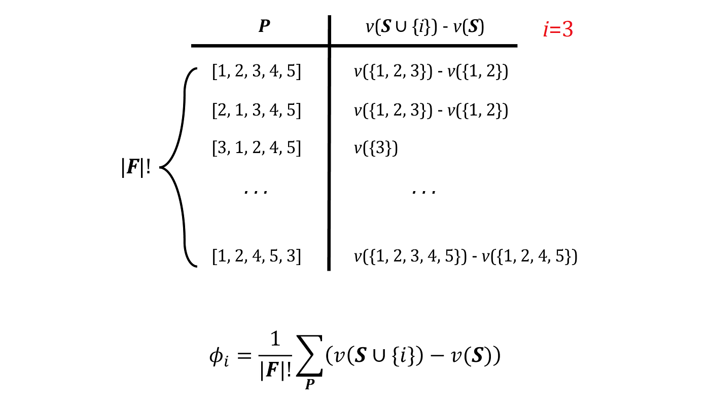
As you see in Figure 3, some permutations have the same contribution since their coalitions S and S U {i} are the same. So, an easier way to calculate Eq. 1 is that we only calculate the distinct values of contributions and multiply them by the number of times that they have been repeated. To do that, we need to figure out how many permutations can be formed from each coalition. Let F-{i} be the set of all players excluding the player {i}, and S is one of the coalitions of F-{i} (S ⊆ F-{i}). For example for F={1,2,3,4,5} and {i}={3}, we have

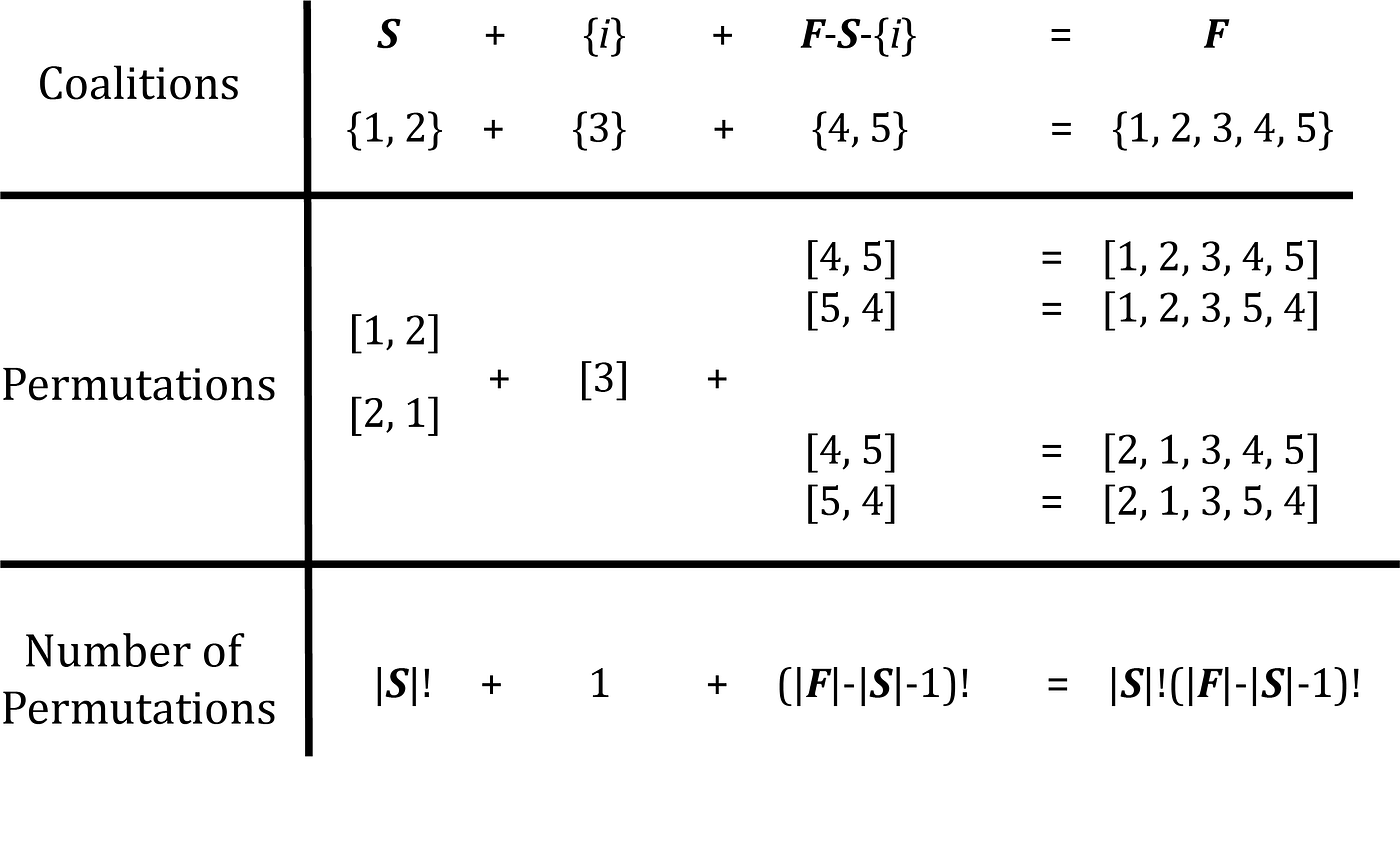
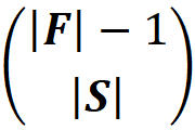
The number of elements in S is denoted by |S|, and we can have |S|! permutations with these elements. For example, if S={1,2} then|S|=2 and we have 2!=2 permutations: [1, 2] and [2, 1] (Figure 4). We also know that the worth of each permutation formed from S is v(S). Now we add the player {i} at the end of each permutation formed from S. The worth of the resulting permutations are v(S U {i}) since they all belong to the coalition S U {i}. The set F has |F|-|S|-1 remaining elements excluding the elements of S U {i} that can be added at the end of S U {i} to form a permutation that has all the elements of F. So, there are (|F|-|S|-1)! ways to add them to S U {i}.
For example, in the previous example the remaining elements of F are {4} and {5}. So we have (|F|-|S|-1)! = (5–2–1)!=2 ways to form the grand coalition using these remaining elements. As a result, we have S! (|F|-|S|-1)! ways of forming a permutation of F in which {i} comes after a permutation of S and the remaining players come after {i} (Figure 4).
The contribution of {i} to the total gain of each permutation is:
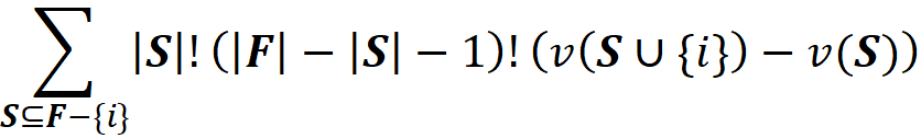
And the total contribution of {i} to the total gain of all these permutations is

So far, we have covered the permutations of one possible coalition S in F and calculated the total contribution of {i} to their total gain. Now we can repeat the same procedure for the other coalitions of F-{i} to get the sum of the contributions of {i} in all the permutations of F:
Finally, we know that we have |F|! permutations for F. So, the average contribution of {i} to the total gain of all the permutations of F can be obtained by dividing the previous term by |F|!
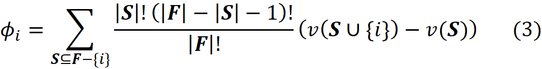
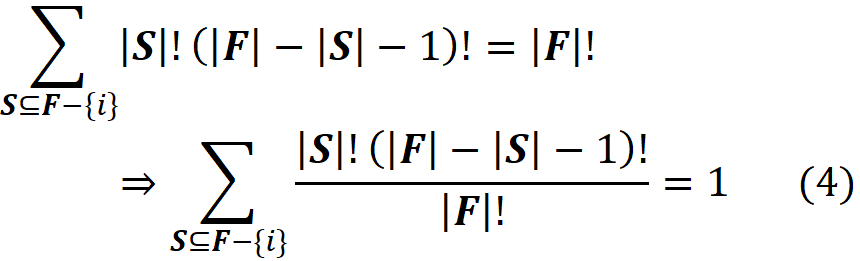
Here ϕᵢ is called the Shapley value of the element {i} which is the average contribution of {i} in all the permutations of F. This is the mathematically fair share of player {i} to the total gain of all the players in F. As we showed before, each coalition S, can make S! (|F|-|S|-1)! permutations. Since the total number of permutations is |F|!, we can write:
The Shapley value should have the following properties:
1- Efficiency: the sum of the contributions of all players should give the total gain:

1- Symmetry: If i and j are such that v(S ∪ {i}) = v(S ∪ {j}) for every coalition S not containing i and j, then ϕᵢ=ϕⱼ .This means that if two players add the same gain to every possible coalition then they should have the same contribution.
2- Dummy: If i is such that v(S) = v(S ∪ {i}) for every coalition S not containing i, then ϕᵢ = 0. This means that if a player doesn’t add any gain to any possible coalition, then its contribution is zero.
3- Additivity: Suppose that u and v are two different characteristic functions for a game. Let the contribution of player i in them be ϕᵢ(u) and ϕᵢ(v) respectively (here ϕᵢ(u) means that ϕᵢ is a function of u). Then we have ϕᵢ(u + v) = ϕᵢ(u) + ϕᵢ(v). Let’s clarify this property by an example. Suppose that a team of employees works on two different projects, and the total payoff and contribution of them to each project is different. Then if we combine these projects, the contribution of an employee in the combined project is the sum of his contributions to each project.
We can easily show that the Shapley values in Equation 3 satisfy these properties.
Proof (optional):
- If for every coalition S, we have v(S) = v(S ∪ {i}) then we get:
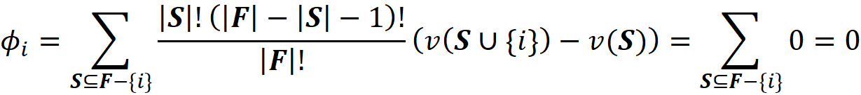
So, they have the dummy property. They also satisfy the efficiency property. From Equation 2 we know that:
where cᵖᵢ denotes the contribution of {i} to the total gain of permutation P. Now suppose that the elements of this permutation are:
So we have|F|=M. We can calculate the values for cᵖᵢ each element:
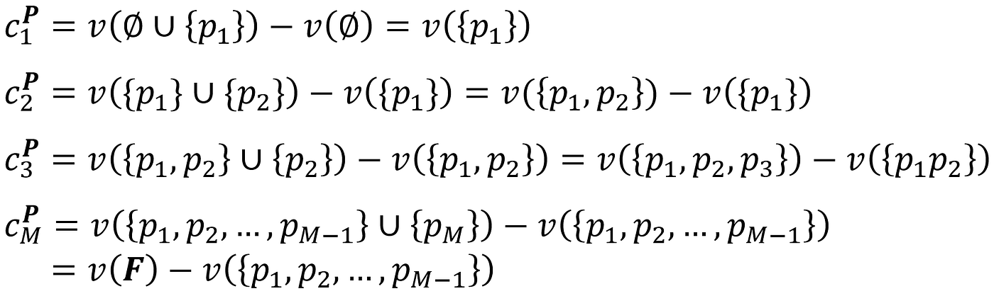
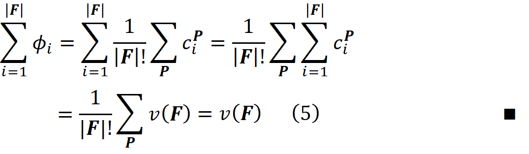
Now if we add the values of cᵖᵢ for all the players, the first term in each cᵖᵢ cancels the second term in cᵖᵢ₊₁ and we get:

So, for each permutation, the sum of the contributions of all players gives the total gain of the grand coalition. We know that we have |F|! permutations. Hence, using Equation 2 we can write:
Shapley values in machine learning
But how can we relate the Shapley value of a player to the features of a machine learning model? Suppose that we have a data set with N rows and M features as shown in Figure 5.
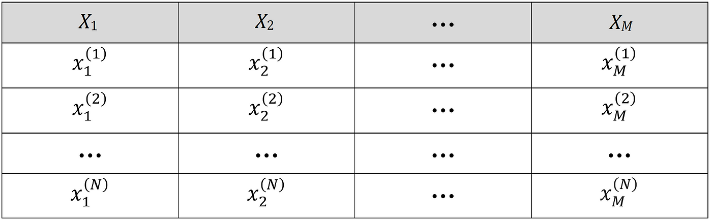
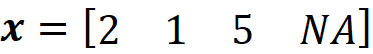
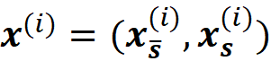
Here Xᵢ is the i-th feature of the data set, xᵢ⁽ʲ⁾ is the value of the i-th feature in the j-th example, and y⁽ʲ⁾ is the target of the j-th row. The values of the features can form a feature vector which is represented by a row vector with M elements:
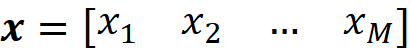
Here we have X₁=x₁, X₂=x₂, … X_M=x_M (in linear algebra the vectors are usually considered column vectors, but in this article, we assume that they are row vectors). A feature vector can be also the j-th row of the data set. In that case, we can write:
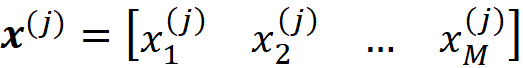
Or it can be a test data point that is not present in the data set (in this article, bold-face lower-case letters (like x) refer to vectors. Bold-face capital letters (like A) refer to matrices, and lower-case letters (like x₁) refer to scalar values). The features of a data set are denoted by capital letters like (X₁). A pair (x⁽ʲ⁾, y⁽ʲ⁾) is called a training example of this data set. Now we can use a model to learn this data set:

The function takes the feature vector x which means that it is applied to all the elements of x. For example, for a linear model we have:

So, for each value of x, the model prediction is f(x). As mentioned before, this feature vector x can be one of the instances of the training data set, or a test data instance that doesn’t exist in the training data set. For example, with this linear model, we can predict the target of one of the training examples:

So, f(x⁽ʲ⁾) is the model prediction for the j-th row of the data set, and the difference between f(x⁽ʲ⁾) and y⁽ʲ⁾ is the prediction error of the model for the j-th training example.
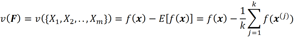
We can assume that a machine learning model is a coalition game, and the M features are the M players in this game. But what should be the characteristic function of this game? Our first guess can be f(x) itself. But remember that a characteristic function should satisfy Equation 1 which means that when we have no players the total gain is zero. How can we evaluate f(x) when we have no features (players)? When a feature is not part of the game, it means that its current value is not known, and we want to predict the model’s target without knowing the value of that feature. When we have no features in the game, it means that the current value of none of the features is known. In that case, we can only use the training set for prediction. Here, we can take the average of f(x⁽ʲ⁾) for a sample of the training examples (or all of them) as our best estimate. So, our prediction when we have no features is:
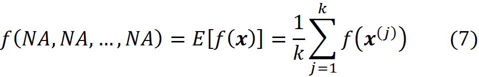
Where NA means a non-available feature (so none of the parameters of f are available here). We also sampled k data instances (feature vectors) from the training data set (k≤N). Now we define our characteristic function for the grand coalition as:
If we have no features, then using Equation 7 we get:

This characteristic function now satisfies Equation 1 and can give the worth of the grand coalition F={X₁, X₂,…, X_M}. But we also need the worth of any coalition of F-{i} to be able to use Equation 3. How can we apply the function f to a subset of its original arguments? We can do it in two ways. First, we can retrain the same model (with the same hyperparameters) only on a subset of the original features. For example, if the coalition S contains the features:
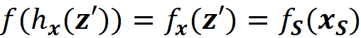
Then we need the marginal value of f for these features which is called fₛ(xₛ):

Here xₛ is a vector that only contains the values of the features present in S (please note that a coalition is composed of the features, but a function takes the values of these features). We can either retrain the same type of model on the features present in the coalition S, to get fₛ(xₛ), or we can use the original function f to calculate fₛ. When a feature is not present in S, then it means that we don’t know its current value, and we can replace it with NA (Not Available).

For example, if F={X₁, X₂, X₃, X₄, X₅}, and the coalition S={X₁, X₂, X₅}, then we don’t know the current value of the features X₃ and X₄. So:

Here we assume that the model represented by f can handle NA values. Hence the worth of this coalition is:

where fₛ(xₛ) is obtained by either retraining the model on the features present in the coalition S or from Equation 9. For example, for F={X₁, X₂, X₃, X₄, X₅} and S={X₁, X₂, X₅}, the worth of S is:

Now we can simply use Equation 3 and Equation 10 to calculate the Shapley value of the feature Xᵢ:

Please note that in this equation, we should have written ϕₓᵢ to be consistent with Equation 3. However, we use ϕᵢ for simplicity. So, in this equation, i denotes the i-th feature (Xᵢ). By simplifying the previous equation, we get:
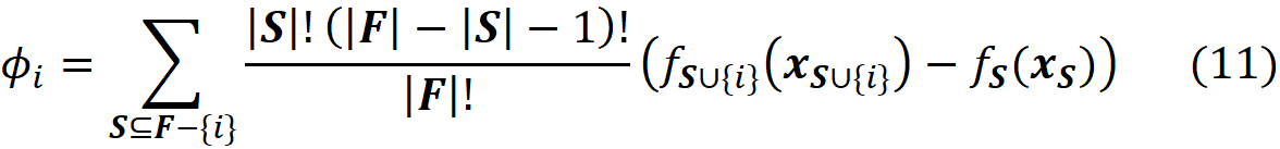
where fₛ(xₛ) is the marginal value of f for the features present in the coalition S, and f_S∪{i}(x_S∪{i}) is the marginal value of f for the features present in the coalition S plus feature {i}. If we use the efficiency property of Shapley values (Equation 5), we can write:
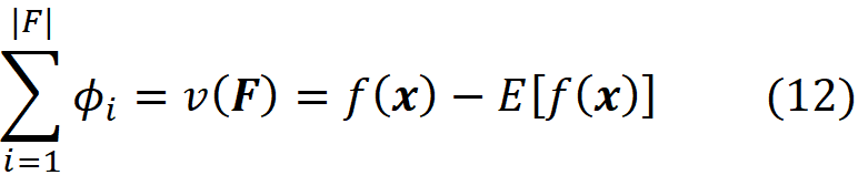
which means that the sum of the Shapely values of all the features gives the difference between the prediction of the model with the current value of features and the average prediction of the model for all the training examples.
The mathematical description of the model explanation
Before discussing the SHAP values, we need to have a mathematical description of an explainer model like SHAP. Let f be the original model to be explained defined as:
So, the model takes the feature vector x and f(x) is the model prediction for that feature vector. This feature vector can be one of the instances of the training data set (x⁽ʲ⁾) or a test feature vector that doesn’t exist in the training data set. Now we create a set of simplified input features to show if a feature in the feature vector is present or not:

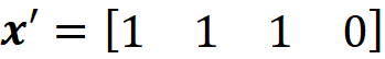
The vector x’ is called a simplified feature vector. Each x’ᵢ is a binary variable that shows if its corresponding feature Xᵢ is being observed in the feature vector (x’ᵢ =1) or it is unknown (x’ᵢ = 0). For, example if your feature vector is
Then
We can assume that there is a mapping function that maps x’ to x:
So, it takes the simplified feature vector x’ and returns the feature vector x:

The explainer is an interpretable model g that takes M binary variables:

Where M is the number of simplified input features in Equation 13. The row vector z’ represents a coalition of the available values of x. So the zero elements of x’ are always zero in z’, and the 1 elements of x’ can be either 1 or 0 in z’. We call z’ a coalition vector. For example, if the values of the features are:

Then the feature vector is:
And the simplified feature is:
Now a value of z’ such as
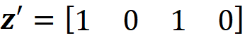
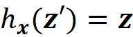
simply represent the coalition S={X₁, X₃} since only these two features have a corresponding 1 in z’. We can also conclude that x’ represents the grand coalition F={X₁, X₂, X₃}, so x’ can be also considered as a coalition vector. As mentioned before, we want the prediction of the explainer model to be close to the prediction of the original model for a single feature vector. Suppose that we start with a coalition vector z’ which is very close to the grand coalition x’. The prediction of g for this coalition is simply g(z’). But how can we get the prediction of f using z’? The problem is that f takes a feature vector, not a coalition vector. So we need the mapping function hx to find the corresponding value of features for z’. Here hₓ(z’) returns the corresponding value of the features that are present in z’, and the value of the other features will be NA. For example, if we have
Then

The prediction of f for the features present in z’ will be:

We also define fₓ to be the marginal value of f for the features present in z’. So we can write:

Please note that in Equation 8, fₛ denoted the marginal value of f for the features present in coalition S. However, here we focus on z’ instead of the coalition, and fₓ denotes the marginal value of f for the features present in z’. In this example, we z’ represents the coalition S={x₁, x₃}. So we can also write:

We want the prediction of f which is f(z) to be very close to that of g which is (g(z’)) to make sure that g mimics the same process that f uses to make a prediction. In summary, we want

to be able to claim that g can explain f.
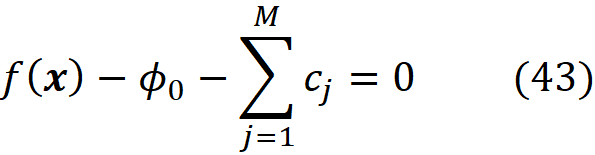
We can classify the explanation methods based on g. Additive feature attribution methods have an explainer model that is a linear function of binary variables:
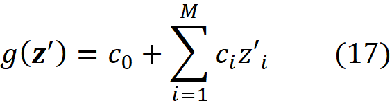
where ci are some constants. As we see later SHAP belongs to this class of methods. So we want to express Equation 11 in terms of z’. Let x be a feature vector, and x’ be its simplified feature vector. We can show that the Shapley values can be expressed as:
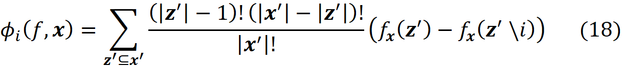
where ϕᵢ(f, x) emphasizes that the Shapley value is a function of f and x. Here we consider all the possible coalition vectors of x’ (which correspond to all coalitions of x). For each coalition vector z’, we calculate the contribution of the feature i. |z’| is the number of non-zero entries in z’ (the size of the corresponding coalition), and |x’| is the number of non-zero entries in x’ (the size of the grand coalition). z’\i means that the corresponding coalition doesn’t include the feature {i}. So, z’\i denotes the coalition vector resulting from setting the i-th element of z’ to 0 (z’ᵢ=0). For example, if 3 represents the 3rd feature x₃, then we can write:

It is easy to show that Equation 11 and Equation 18 are equivalent.
Proof (optional): First, note that |F| in Equation 11 is equal to |x’| in Equation 18 since they both refer to the total number of features, M. Remember that each coalition S in Equation 11 doesn’t include the feature i since S ⊆ F-{i}. We can easily see that each coalition S in Equation 11 has a corresponding value of z’\i in Equation 18. For example, if we have:

Then we get:

And the corresponding value of z’\i for S is [1 1 0 0 1].

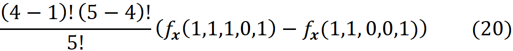
By replacing these values in Equation 11, the corresponding term for this value of S is:

In Equation 18, the corresponding term for this value of z’ is:
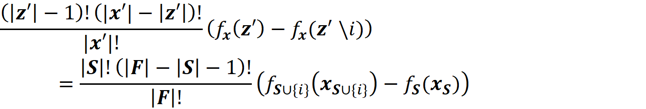
Now based on Equation 15, we conclude that Equation 19 and Equation 20 give the same result. Generally, for each coalition S in Equation 11, we have a z’\i that represents it. As a result, z’ also represents S ∪ {i}, and we can replace fₛ(xₛ) and f_S∪{i}(x_S∪{i}) with fₓ(z’) and fₓ(z’\i) respectively. In addition, |S| and |F| are equal to |z’|-1 and |x’|. Hence each term in Equation 11 (for a coalition S that doesn’t include i) has a corresponding term in Equation 18 in which the coalition vector z’ includes I, and both terms give the same value:
But this only covers the z’s in Equation 18 that include {i}. In Equation 18, we can also have z’s that don’t include {i}. For a coalition vector z’ that doesn’t include {i}, we can write fₓ(z’)=fₓ(z’\{i}), so its corresponding term in Equation 18 is zero
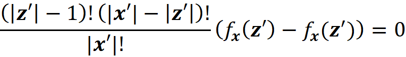
and it doesn’t add anything to Equation 18. Hence, we conclude that Equation 11 and Equation 18 are equivalent and give the same result. ∎
It is important to note that in Equation 18, the coalition vector of the empty coalition (z’=[0 0 … 0]) is not included in the sum. For this coalition vector we have:
which is not defined. Even if could calculate it, this coalition wouldn’t add anything to this sum since
Please also note that in the original paper that introduced the SHAP method, Equation 18 is not written correctly (refer to equation 8 in [1]). Equation 11 is the classic Shapley value equation, and in this equation, we only focus on the available features. Equation 18 introduces the concept of missingness. Here the grand coalition vector x’ can have some missing values for which x’ᵢ=1. Equation 18 has some interesting properties which are described below:
Property 1 (Local accuracy)
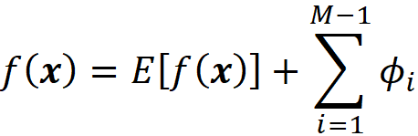
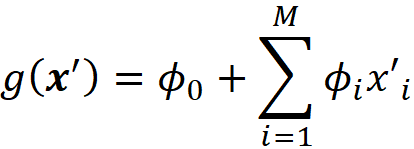
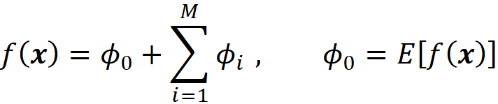
Let g(x’) be an explanation model defined as
where ϕ₀ =E[f(x)], and ϕᵢ are the Shapley values of f. Suppose that we have a feature vector x and its simplified feature vector is x’, so we have x = hₓ(x’). Then based on this property, the prediction of g for x’ matches the prediction of the original model f for x. So, we can write:
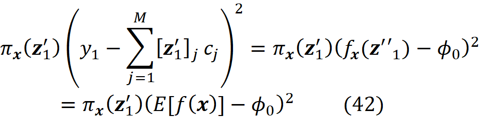
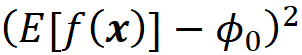
Proof (optional): Assuming that |F|=M (number of features), and all features are available (x’ᵢ=1 for all i) we can use Equation 12 to write:

where ϕ₀ =E[f(x)]. ∎
As mentioned before Equation 11 only considers the available features. Since Equation 12 is derived from this equation, it only includes the Shapley values of the available features. For example, if the last feature is unavailable, then from Equation 12 we get
However, this result is still consistent with Equation 22 since for the last feature we have x’_M=0.
Property 2 (Missingness)
A missing feature should have a zero Shapley value.
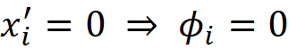
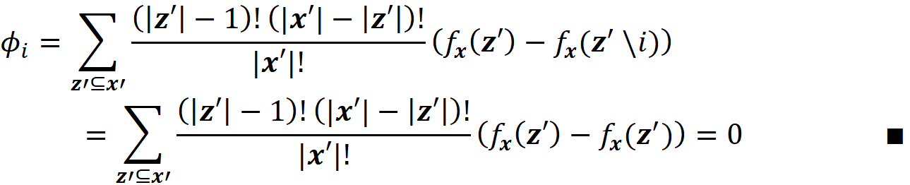
Proof (optional): This is not a necessary condition for the classic Shapley values in Equation 11. Since it doesn’t include the missing features. However, if we calculate the Shapley values using Equation 18, then we can show that it satisfies this property. Consider all the coalitions vectors z’ derived from x’. If x’ᵢ=0, then z’ᵢ =0. So, for these coalition vectors we get z’\i=z’, and we can write:
Property 3 (Consistency)
Consistency means that changing the original model to increase the impact of a feature on the model will never decrease its Shapley value. Mathematically, if we have a single feature vector x, and two models f and f’ (both f and f’ are a function of x) so that

for all inputs z’, then
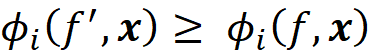
Remember that in Equation 18, the term
is proportional to the contribution of feature Xᵢ to the prediction. So if change the model from f to f’ and get a higher contribution of the feature Xᵢ to the prediction of x increases (or remains the same), then the Shapley value of Xᵢ never decreases.
Proof (optional): Again, it is easy to show that Equation 18 satisfies this property. Since we have the same feature vector x for both models, we will have the same x’. Now for each coalition vector z’ of x’ we have
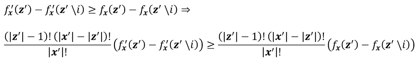
So, by adding these terms for all z’ we have:
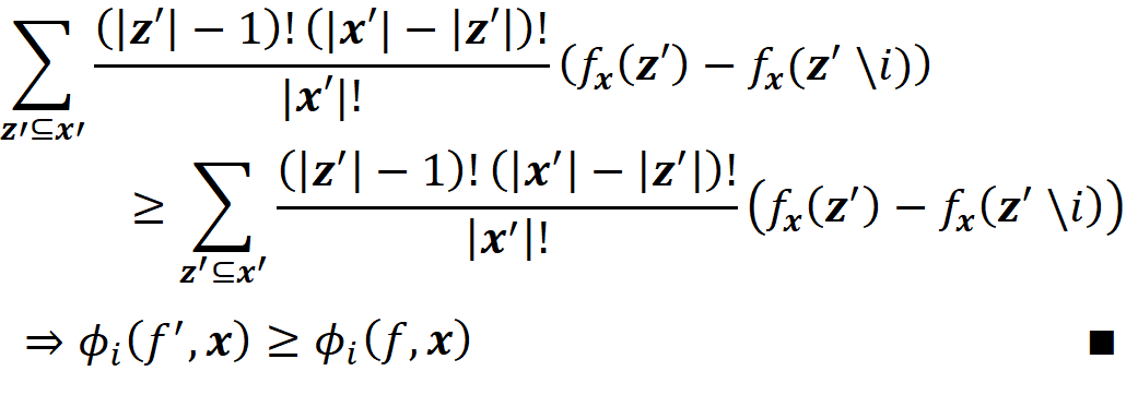
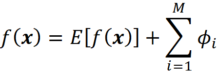
Now that we are familiar with Shapley values and their properties, we can see how they can explain a machine learning model. Suppose that we have a model f, and a feature vector x. We define the model g as:
where ϕ₀ =E[f(x)], ϕᵢ are the Shapley values of f, and x’ is the simplified feature vector of x (so x = hₓ(x’)). The model g is linear, so it is interpretable. In addition based on property 1, g(x’)=f(x), so g can mimic f perfectly for a single prediction f(x), and can be used as an explainer model for f. It can be shown that for an additive feature attribution method, the model g defined above is the only possible explainer model that follows Equation 17 and satisfies the properties 1, 2, and 3. In summary, the Shapley values can provide the coefficients of a linear model that can be used as a perfect explainer for any machine learning model.
From Shapley values to SHAP values
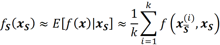
Shapley values have a solid theoretical foundation and interesting properties, however, in practice, it is not easy to calculate them. To calculate them we need to calculate fₓ(z’) in Equation 18 or fₛ(xₛ) in Equation 11. Remember that
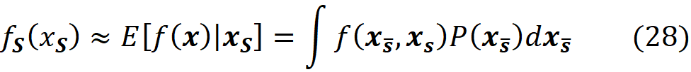
So, calculating fₓ(z’) or fₛ(xₛ) means that we need to calculate f(x) with some missing features which are not included in z’ or S. The problem is that most models cannot handle missing values. For example, in a linear model, we need all the values of xᵢ to calculate f(x). So, we need a way to handle the missing values in f(x). As mentioned before, for each coalition S, the missing elements of x are the values of features that are not present in S. To calculate fₛ(xₛ), we assume that:

Here E[f(x)|xₛ] is the expected value of the f(x) conditioned on the features present in S. Similarly, we can write:

The Shapley values calculated using the conditional expectations in Equation 23 or Equation 24 are called SHAP (SHapley Additive exPlanation)) values. So, to get the SHAP values from Equation 11 we can write:

And to calculate the SHAP values from Equation 18 we can write:

SHAP is an additive feature attribution method in which we have a linear explainer model. In this paper, we discuss two methods to calculate the conditional expectations in Equation 23 or Equation 24. The first one is discussed in this section, and the second one which is suitable for tree-structured data will be discussed later.
Let S̅ denote the complement of the coalition S. So, x_S̅ denotes part of the original features which are not present in S. Now we can use the law of total probability to write:

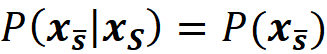
where f(x_S̅, xₛ) denotes that some of the parameters of f belong to xₛ and the remaining parameters belong to x_S̅ . Of course, the parameters of xₛ or x_S̅ are not necessarily arranged consecutively. P(x_S̅|xₛ) is the conditional probability of x_S̅ given xₛ. So, to compute the value of fₛ(xₛ), we need the conditional probability P(x_S̅|xₛ). Unfortunately, we don’t know this distribution most of the time. Hence in SHAP, we assume that the features are independent of each other, So:
By replacing this equation in Equation 27, we get:
Since we have discrete data points, we can approximate this integral with a sum. We sample k data instances (feature vectors) from the training data set (k≤N) and call each of them x⁽ʲ⁾. The features in each data instance either belong to S or S̅:
Then for each data instance, we replace the values of the features that are present in S with their corresponding values in xₛ, and make the prediction for that data instance:
Now the previous integral can be approximated with the average value of these predictions:
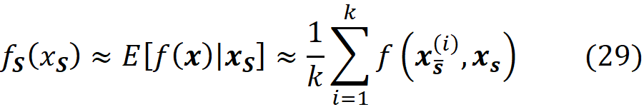
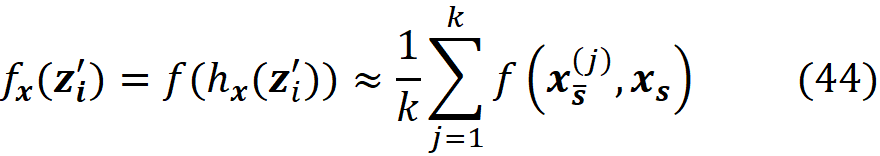
Figure 6 shows an example of calculating this integral. Similarly, we can write:
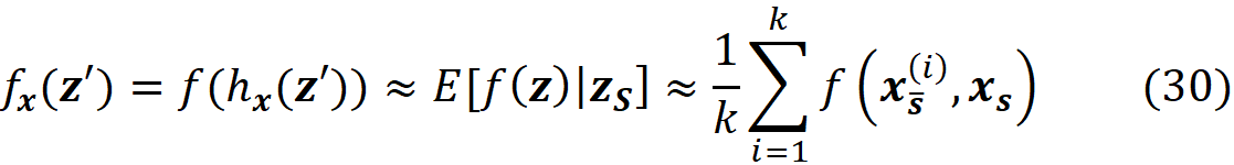
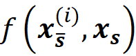
where zₛ is the set of features that have a non-zero index in z’. Figure 6 shows an example of this method. Here we have a model f(x₁, x₂, x₃, x₄, x₅) in which xₛ ={x₁, x₃, x₄}. So x_S̅ ={x₂, x₅} and the features X₂ and X₅ are NA in x. The feature vector x is in the form of x=[ x₁ NA x₃ x₄ NA]. To calculate f(x), we need a value for the missing features, so we borrow the value of them from a sample of the training data set. For the i-th data instance of this sample, we replace the missing values of the feature vector x (X₂, X₅) with their corresponding value in that instance (x₂^(i), x₅^(i)), and calculate f(x_S̅^(i), xₛ) = f(x₁, x₂^(i), x₃, x₄, x₅^(i)). So for each data instance, we have a prediction now. Finally, we take the average of these predictions and report it as our estimation of f(x). Now we can use the approximations given in Equation 29 and Equation 30 to calculate the SHAP values in Equation 25 or Equation 26.
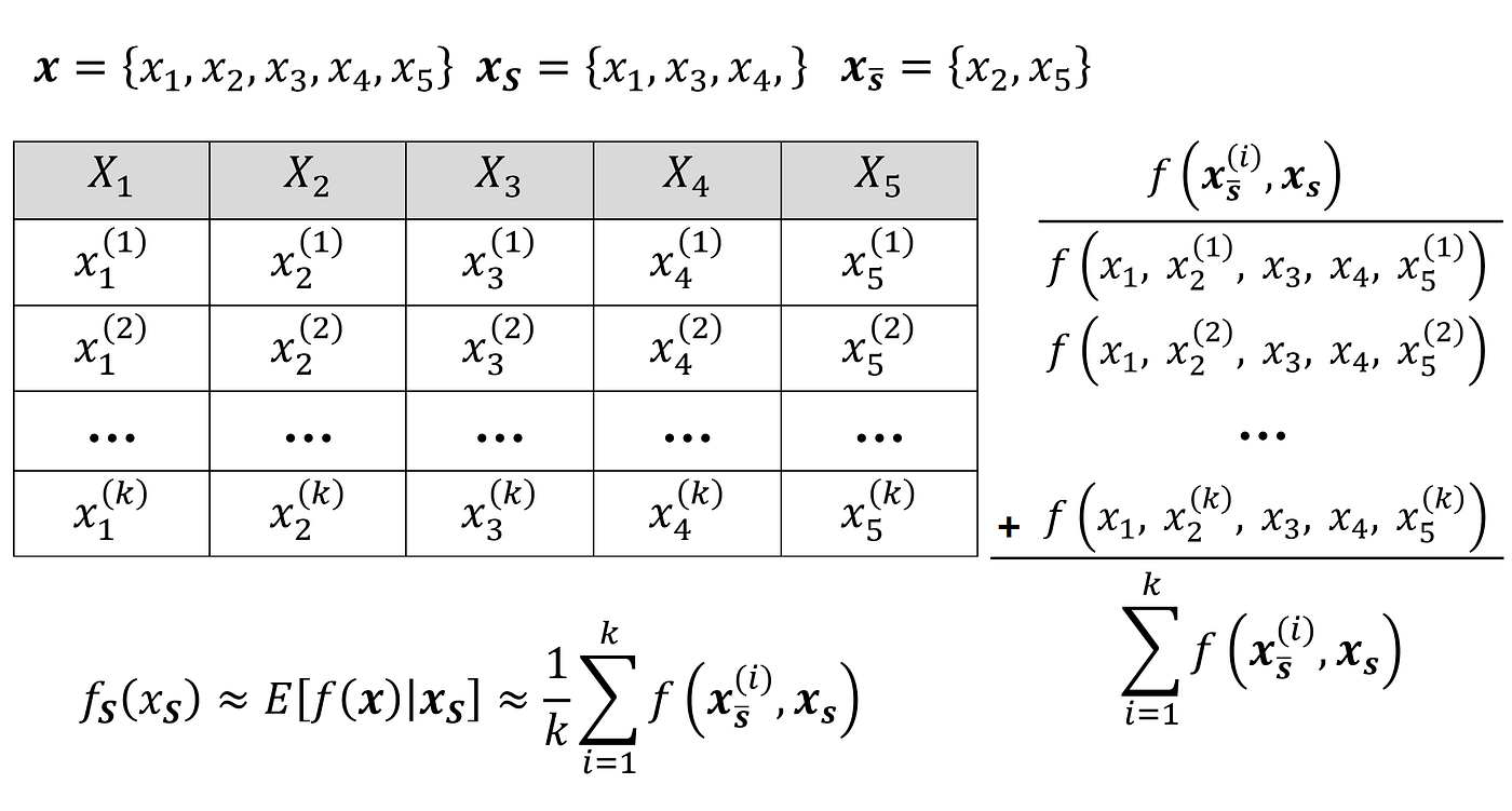
Please note that Equation 30 is also consistent with Equation 7. When all the elements of z’ are zero, S becomes an empty set, so we only take the average value of the model prediction for the k data instances of the training set.
Linear SHAP
Suppose that our predictive model f is a linear regression model:

where x₀=1, and the features Xᵢ, i = 1, …, M are independent. Now we can show the SHAP values are given by the following equation:

Where k is the number of data instances in a sample of the training data set that we use to calculate the SHAP values. You can refer to the appendix for the proof. We can also drive this equation intuitively. In a linear model, the contribution of the feature Xᵢ to f(x) is simply cᵢxᵢ. So we could write:
However, Equation 22 adds a constraint to the Shapley values:
So we subtract
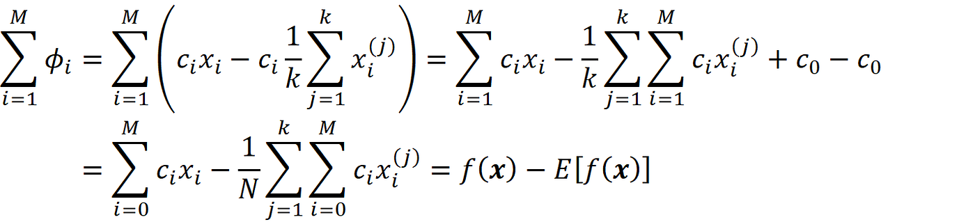
from cᵢxᵢ in Equation 31 to satisfy Equation 22. If we add the Shapley values from Equation 31, we see that the result is consistent with Equation 22:
Calculating SHAP values in Python
Linear SHAP
As our first example, we use Python to calculate the linear SHAP values (Equation 31) for a dummy data set. We first define the data set. We only have two features filled with some random numbers, and the target is defined as a linear combination of these features. The features are independent.
# Listing 1# Defining the dataset
X = pd.DataFrame({'a': [2, 4, 8, 0, 3, 6, 9],
  'b': [1, 5, 0, 7, 1, -2, 5]})
y = 5*X['a'] + 2*X['b'] + 3
Then we use a linear regression model for this data set and calculate the coefficients of this model which are the same coefficient used to define the target.
# Listing 2# Defining a linear model
linear_model = LinearRegression()
linear_model.fit(X, y)print("Model coefficients:")
for i in range(X.shape[1]):
   print(X.columns[i], "=", linear_model.coef_[i].round(4))
Output:
Model coefficients:
a = 5.0
b = 2.0
Finally, we use Equation 31 to calculate the SHAP values for the first example of this data set:
# Listing 3shap_values = ((X[:1] — X.mean()) * linear_model.coef_)
shap_values_table = shap_values.T
shap_values_table.columns = ['SHAP_value']
shap_values_table
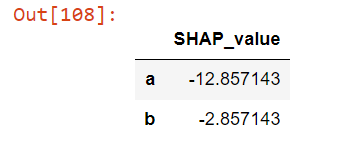
So, we have:
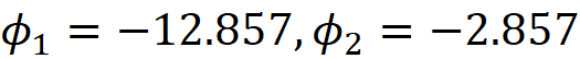
where 1 and 2 refer to the features a and b respectively.
Linear SHAP using the SHAP library
We can also use the SHAP library to calculate the SHAP values of the linear model defined in Listing 2:
import shap
explainer = shap.LinearExplainer(linear_model, X)
shap_values = explainer.shap_values(X[:1])
shap_values
Output:
array([[-12.85714286, -2.85714286]])The class LinearExplainer() in the SHAP library takes the trained model and the training data set. The method shap_values() in this class, takes the array of the rows to be explained and returns their SHAP values. Please note that here we get the same result as Listing 3.
Exact SHAP values
In the next example, we calculate the SHAP values for a linear model with feature dependence. So, we cannot use Equation 31. Instead, we use Equation 11 and calculate the SHAP values using all the possible coalitions. Here we use the Boston data set in the scikit-learn library:
# Listing 4d = load_boston()
df = pd.DataFrame(d['data'], columns=d['feature_names'])
y = pd.Series(d['target'])
X = df[['LSTAT', 'AGE', 'RAD', 'NOX']]
X100 = X[100:200]linear_model2 = LinearRegression()
linear_model2.fit(X, y)
The Boston data set has 13 features, but we only pick 4 of them (LSTAT, AGE, RAD, NOX). We also sample 100 rows of this data set to estimate fₛ(xₛ) in Equation 29 (So k=100). We store these rows in X100. Then we use this data set to train a linear model. Now we need to define some functions to calculate the SAHP values in Python:
The function coalition_worth() is used to calculate the worth of a coalition. It takes a model, a sample of the training data set (X_train), a data instance (x), and the set of coalitions (coalition). Here coalition represents S in Equation 11. This function replaces the columns of X_train with the values given in the coalition set, and then it uses the model to predict the target of all these rows. Finally, it takes the average of all these predictions and returns it as the estimation of fₛ(xₛ).
The function coalitions() returns the set of all coalitions of a data instance excluding the feature col. So, it calculates all the coalitions of F-{i} in Equation 11, where col represents the feature i.
The function coalition_contribution() calculates the contribution of each coalition in Equation 11 (each term of the summation in Equation 11). Here we used the fact that:

So the function comb() in scipy has been used to calculate the binomial coefficient:
Finally, the function calculate_exact_shap_values(), takes the feature vectors to be explained (X_explain) and calculates the SHAP values of each feature vector in that. It adds the contribution of each coalition to calculate the SHAP value of each feature in a feature vector. Now we can use this function to calculate the SHAP values of the first row of the Boston data set using a sample of the data set rows (X100):
# Listing 6calculate_exact_shap_values(linear_model2, X100, X.iloc[0])
Output:
(22.998930866827823,
 [[7.809214247585507,
   -0.7308440229196315,
   0.1290501127229501,
   0.23758951510828266]])
Calculating SHAP values using the SHAP library
The class Explainer() in the shap library takes the model predictor function (not the model alone) and the training data set, and the method shap_values() returns the SHAP values. If we don’t pass the name of a specific algorithm, it attempts to find the best algorithm to calculate the SHAP values based on the given model and the training data set. Here we use it for the same model defined in Listing 4.
explainer = shap.Explainer(linear_model2, X100)
shap_values = explainer.shap_values(X.iloc[0:1])
shap_values### Output:
array([[ 7.80921425, -0.73084402,  0.12905011,  0.23758952]])
explainer.expected_value### Output:
22.998930866827834
Here the array shap_values give the values of ϕ₁ to ϕ_M. The value of ϕ₀ is stored in the field expected_value in Explainer. Here we get almost the same SHAP values that calculate_shap_values() in Listing 6 returned. It is important to note that the Explainer class automatically samples 100 rows of the training data (if the number of rows is greater than 100) and uses that to calculate the SHAP values. So if we use a training data set which has more than 100 rows, the output of Explainer won’t match the output of calculate_exact_shap_values() anymore:
explainer = shap.Explainer(linear_model2, X[:150])
shap_values = explainer.shap_values(X.iloc[0:1])
shap_values### Output:
array([[ 8.88370884e+00, -2.97655621e-01,  1.17561972e-01,
        -1.48202335e-03]])
calculate_exact_shap_values(linear_model2, X[:150], X.iloc[0])### Output:
(22.521908424669917,
 [[7.993180897252836,
   -0.11946396867250808,
   0.11973195423751992,
   -0.07141658816282939]])
Kernel SHAP
To calculate the SHAP values of a model using Equation 11 or Equation 18 we need to calculate all the possible coalitions. As mentioned before, for M features, the total number of possible coalitions is 2 . Of course, In Equation 25 we calculate all the coalitions of F-{i}. So, the actual number of coalitions that we need to calculate each SHAP value is 2ᴹ⁻¹, and for M features the time complexity is
For each coalition, we need to estimate fₛ(xₛ) and f_S∪{i}(x_S∪{i}) using Equation 29, and in this equation, we take the average of k samples. So time complexity of this algorithm is O(kM2ᴹ).
Based on this result, the number of possible coalitions increases exponentially when M increases, and finding the SHAP values using these equations becomes computationally intractable when we have more than a few features. Kernel SHAP is an approximation method that can be used to overcome this issue. This method was first developed by Lundberg and Lee [1].
LIME
To understand the kernel SHAP, we should first get familiar with another model-agnostic explanation method called LIME (Local Interpretable Model-agnostic Explanations). LIME was developed before SHAP, and its goal was to identify an interpretable model for a classifier that is locally faithful to it. Suppose that you have a model f(x) and you want to find the best interpretable model g(z’) for that (remember that g is a function of the coalition vector z’). Let x be the feature vector to be explained, and x’ be its coalition vector.
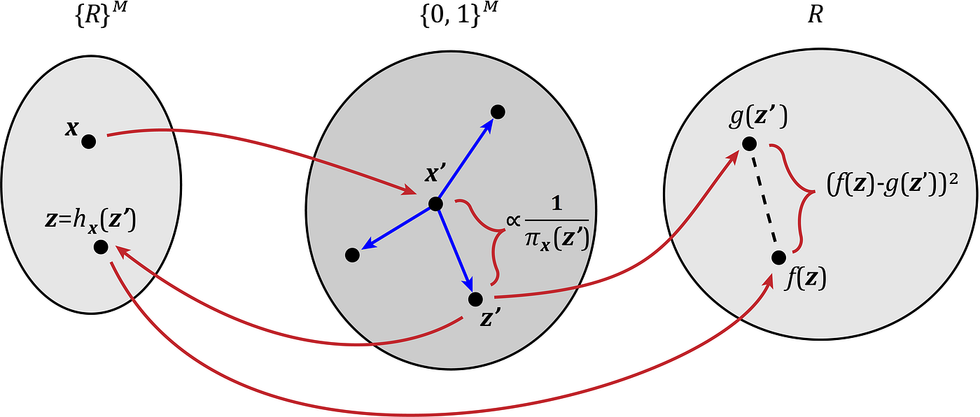
Now we need to find some random coalition vectors near x’. For, example, we can select some non-zero components of x’ and change them from 1 to 0 with a probability of 0.5 to produce the coalition vector z’. As a result, we end up with some coalition vectors near x’. We generally call each of these coalition vectors, z’, and we call the set of all these vectors Z. We can assume that x’ and z’ are some points in an M-dimensional space (Figure 7). We can use the mapping function hₓ to find the corresponding vector of each z’ in the feature space (Figure 7):
We need to have a quantitative measure of the distance between x’ and each z’. So, we defined the function πₓ(z’) as a measure of the distance between x’ and z’. This function maps the coalition vector z’ to a non-negative real number ({0,1}ᴹ → R≥ 0). πₓ(z’) should increase as z’ gets closer to x’.
Now suppose that we have a set of interpretable explainer models G, and we want to find the most accurate explainer model g for f(x) among them (g ∈ G). From Equation 16, we want to have:

As a result, we can define a loss function L(f, g, πₓ) that is proportional to the distance between f(z) and g(z’) for all vectors z’ in Z. We want g(z’) to be very close to f(z) when z’ is very close to x’. However, some of the points in Z may not be very close to x’, so we need to add a penalty term for them. Since πₓ is a measure of the distance between x’ and z’, we can add it as a parameter to the loss function. For example, we can define the loss function as:
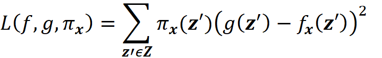
By adding πₓ to the loss function, we add a higher penalty for the points in Z which are far from x’, and the closer points become more important for minimization. Hence, the loss function determines how poorly an explanation function g approximates f at the points z’ which are very close to x’. Now we need to find function g in G (set of all interpretable functions that we want to try), that minimizes this loss function.
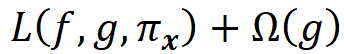
We also favor the functions that are simpler and more interpretable, so we let Ω(g) be a measure of complexity (as opposed to interpretability) of the explanation function g. For example, for linear models, Ω(g) can be defined as the number of non-zero weights, or for decision trees, it can be the depth of the tree. So Ω(g) decreases as g becomes simpler and thus more interpretable, and we should look for a function g in G that minimizes the following objective function:
This is equivalent to solving this minimization problem:
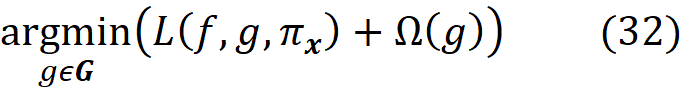
Now we can use the following theorem to define the kernel SHAP method:
Theorem 1. Suppose that we have a feature vector x with M features and a model f which takes x as input. Let g be a linear model defined as:
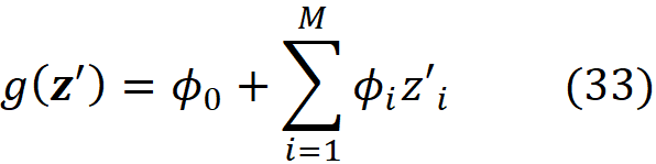
where z’ᵢ is the i-th element of z’ which is a coalition vector of x; ϕ₀ =E[f(x)] (the average prediction of the model for the instances of a sample of the training data set) and ϕᵢ (for i>0) are the Shapley values of f and x defined in Equation 18. As M goes to infinity, the solution of Equation 32 (the function g) approaches the function given in Equation 33, if L, Ω, πₓ are defined as:
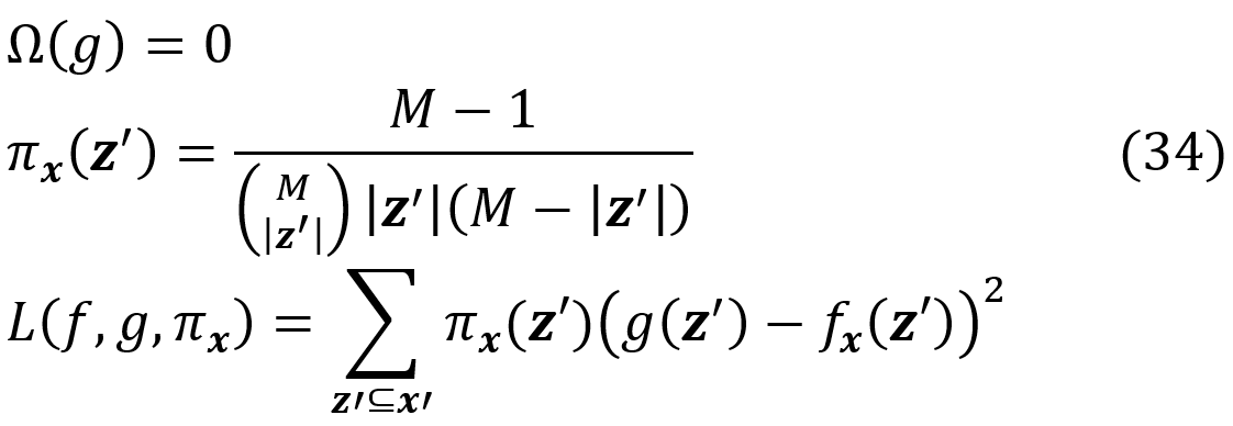
where |z’| is the number of non-zero entries in z’.
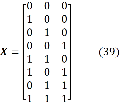
The proof of this theorem is given in the appendix. It is interesting to note that in the original paper that introduced SHAP [2], this theorem wasn’t proved correctly (please refer to the appendix for more details). Let’s see how we can use this method in practice. We assume that we have a feature vector x with M features. We calculate the simplified feature vector x’. Here we assume that there are no NAs in x for simplicity (in theorem 1, x can have NA values), so all the elements of x’ are 1. Then we calculate all the possible coalition vectors of x’ (they are also called a perturbation of x’). Each coalition vector of x’ is called z’ᵢ and is a vector with M elements in which each element can be either 0 or 1. We have 2ᴹ coalition vectors, and we place all these coalition vectors in a 2ᴹ× M matrix X:
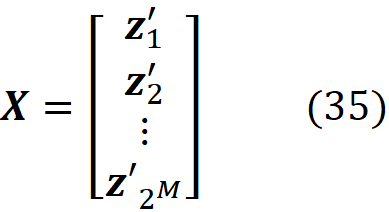
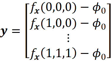
This matrix is called the coalition matrix. For each coalition vector z’ᵢ , we can calculate the model prediction fₓ(z’ᵢ). We define the column vector y as:
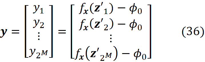
where ϕ₀ =E[f(x)] (the average of the predictions of the data instances in a sample of the training data set).
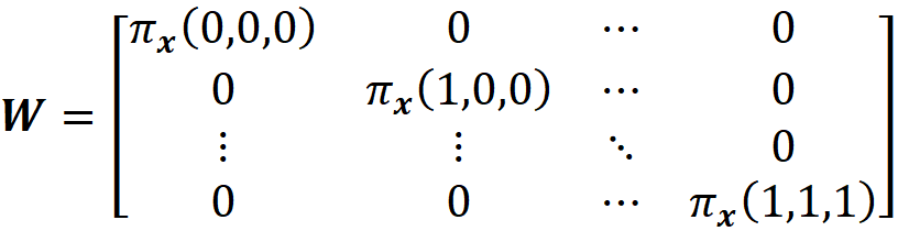
Finally, we define the 2ᴹ× 2ᴹ diagonal matrix W as:
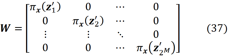
where
For example, let the feature vector be:
Then we have:
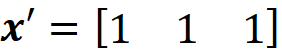
And the coalition matrix will have 2³=8 rows:
And we have:
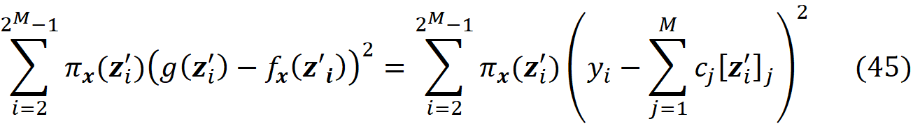
From equations Equation 32 and Equation 34, we know that we need to solve this minimization problem to get an estimation of the Shapley values:
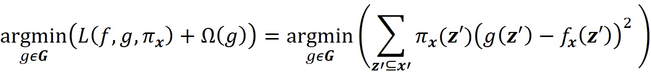
We limit our search for the optimal function g to linear functions with this form:
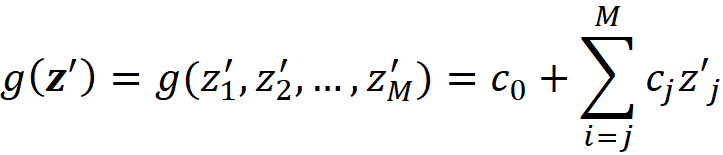
The column vector c is defined as:

Now it can be shown that (the details are given in the appendix):
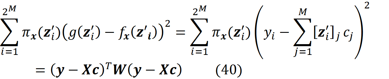
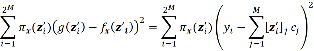
So, the minimization problem is equivalent to
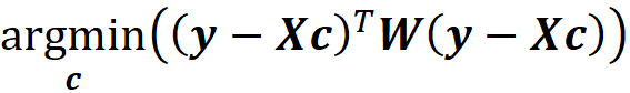
g is only a function of cᵢ, so instead of finding the function g that minimizes the objective function, we find the value of the vector c that minimizes it. The function πₓ(z’ᵢ) is also called the Shapley kernel weight. Based on (Equation 40), each value of πₓ(z’ᵢ) is like a weight for (g(z’ᵢ)-fₓ(z’ᵢ))² and since this term is only a function of z’ᵢ, it is also a weight for the coalition vector z’ᵢ that shows how important a coalition is.
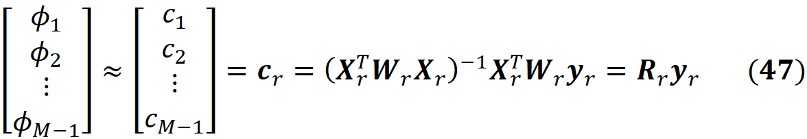
As shown in the appendix, the solution to this minimization problem is:
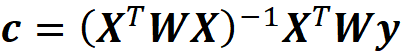
From theorem 1 we know that this solution is an approximation of the Shapley values:
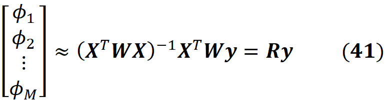
Since ϕ₀ =E[f(x)], we have all the Shapley values. The term R in Equation 41 does not depend on a specific data instance to be explained, so if we want to explain multiple data instances, we only need to calculate R once. Then for each data instance, the new value of y is calculated and multiplied by R to get the SHAP values.
It is important to note that the order of the coalition vectors in X is not important. For example, in Equation 39 the coalition vector [0 0 0] is the first row of X, however, it can be the last row and Equation 41 is still valid (if you look at the proof of theorem 1 in the appendix, we don’t make any assumption about the order of coalition vectors z’ᵢ as the rows of matrix X. It only needs to have all the 2ᴹ coalition vectors.
Kernel SHAP in Python
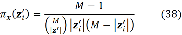
Theorem 1 is valid even if the feature vector x has some non-available features, but in practice, we implement SHAP assuming that all the features of x are available. So, all the elements of x’ are one, and |x’|=M. Now let’s see how we can implement kernel SHAP in Python. To do that, we first need a Python function to calculate πₓ(z’ᵢ).
The function pi_x() takes a coalition vector z’ᵢ (as a list) and returns the values of πₓ(z’ᵢ) based on Equation 38. The function generate_colaition_vectors() takes the number of features (num_features) and generates all the possible coalition vectors for them.
For example:
generate_coalition_vectors(num_features)Output
[[0.0, 0.0, 0.0],
 [1.0, 0.0, 0.0],
 [0.0, 1.0, 0.0],
 [0.0, 0.0, 1.0],
 [1.0, 1.0, 0.0],
 [1.0, 0.0, 1.0],
 [0.0, 1.0, 1.0],
 [1.0, 1.0, 1.0]]
Now we need a function to generate the diagonal elements of the matrix W in Equation 37. Here we have a problem. By looking at Equation 38, we see that if |z’ᵢ |=0 (when all the elements of z’ᵢ are zero) and |z’ᵢ|=M (when all the elements of z’ᵢ are one), then πₓ(z’ᵢ)=∞. Remember that we want to minimize the following objective function (Equation 40):
Let’s assume that the first z’₁ is the coalition in which all the elements are zero:
And let the last coalition be the coalition in which all the elements are one:
We know that when we have no available features, the model prediction is the average of the predictions of the instances in a sample of the training data set (Equation 7). So, we have:
We also know that when all the features are available:

So, for the last coalition we have:
Now in Equation 42, πₓ(z’₁) is the weight of this term:
Since πₓ(z’₁) is infinite, we need this term to be zero, which means that we should have:
which is the property of a linear model based on Shapley values (Equation 22). The infinite value of πₓ(z’_2ᴹ) means that we should have:
We also know that as M goes to infinity, the values of cⱼ that minimize the objective function are getting closer to the Shapley values of f and x. So, the equation above is simply showing the property of a linear model based on Shapley values (Equation 22). Now let’s plot πₓ(z’ᵢ) for a special case where M=13. We can use Listing 9 for this purpose:
# Listing 9pi_values = [1e7]
for i in range(1, 14):
    try:
        pi_values.append(pi_x(13, i))
    except:
        pi_values.append(1e7)
plt.plot(pi_values, marker=’o’)
plt.xlabel(“$|\mathregular{z}’_i|$”, fontsize=14, weight=”bold”,
   style=”italic”,)
plt.ylabel(“$\pi_\mathregular{x}(\mathregular{z}’_i)$”, fontsize=14,
   weight=”bold”, style=”italic”,)
plt.ylim([0, 0.1])
plt.show()
The result is shown in Figure 8. We have used a large constant (1e7) instead of infinity for πₓ(z’₁) and πₓ(z’_2ᴹ) to be able to plot them.
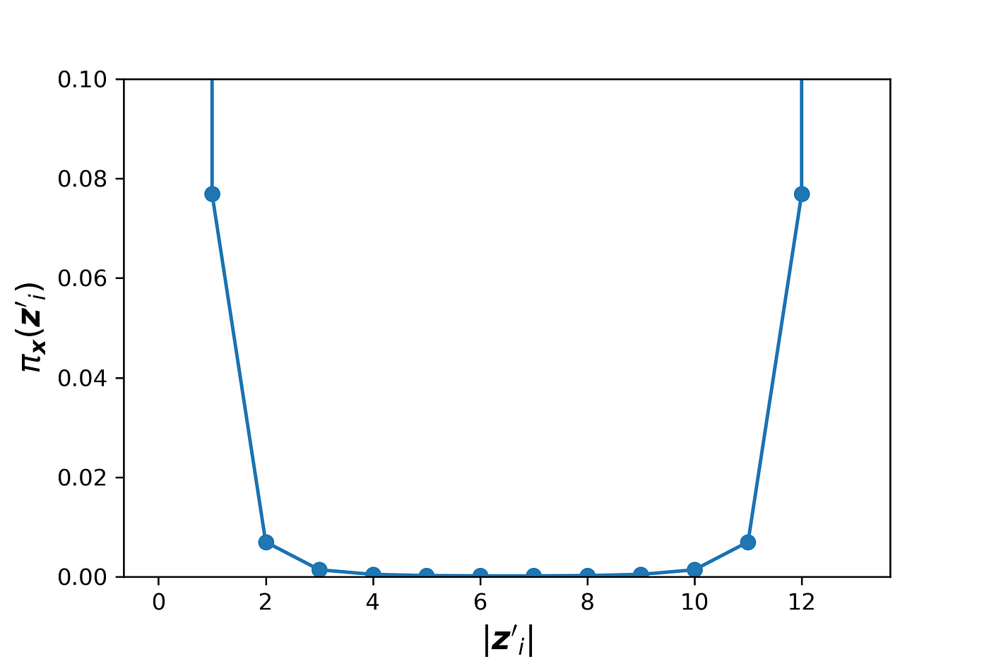
The plot is symmetrical, and as |z’ᵢ| gets closer to 0 or M, πₓ(z’ᵢ) increases. Each value of πₓ(z’ᵢ) is like a weight for the coalition vector z’ᵢ. As mentioned, before we use Equation 30 to estimate fₓ(z’). For z’₁ we know that

And for z’_2ᴹ we know that
These two coalition vectors are the most important ones since we can exactly calculate the value of fₓ(z’ᵢ) for them. Hence they have infinite weights. However, for other coalitions (z’ᵢ) we can only estimate fₓ(z’ᵢ). When the coalition z’ᵢ gets closer to z’₁ or z’_2ᴹ, πₓ gives a much higher weight to it.
The function generate_pi_values() generates the diagonal elements of W. For each coalition vector z’ᵢ, this function calculates πₓ(z’ᵢ) using pi_x(). We cannot use pi_x() for z’₁ and z’_2M since it ends up with a division by zero exception. Instead, we replace πₓ(z’ᵢ) with the large constant 1e7 for the coalitions in which |z’ᵢ|=0 and |z’ᵢ|=M.
Then we need a Python function to calculate fₓ(z’ᵢ) for each coalition vector. We can use Equation 30 for this purpose. Suppose that our feature vector that should be explained is x. We gather all the features in x which are present in z’ᵢ in a set called xₛ. Then for each data instance in the sample of the training data set, we replace the values of the features that are present in S with their corresponding values in xₛ, and make a prediction for that data instance:
We take the average value of these predictions for all the instances of the training set as an approximation for fₓ(z’ᵢ):
The Python function f_x_z_prime() uses this method to calculate fₓ(z’ᵢ) for each coalition vector:
The function kernel_shap() takes a model predictor, the training data set, its weight array and the feature vectors to be explained by kernel SHAP (X_explain). It generates the coalitions vectors, E[f(x)], and the diagonal elements of the matrix W. Then it calls the function calculate_shap_values() to calculate the SHAP values of each feature vector in X_explain. For each feature vector to be explained, this function calculates the SHAP values using Equation 41. It forms the matrices X and W and the column vector y. Then uses Equation 41 to calculate ϕ₁ to ϕ_M. It returns a tuple in which the first element is ϕ₀, and the second element is an array of the SHAP values (ϕ₁ to ϕ_M) of each feature vector in X_explain.
Now let’s try kernel_shap() on a data set. We use the Boston data set again and we include all the features (13 features). Then we train a random forest regressor on that.
# Listing 13d = load_boston()
df = pd.DataFrame(d['data'], columns=d['feature_names'])
X = df[['AGE', 'RAD', 'TAX', 'DIS', 'RM', 'LSTAT', 'B', 'INDUS',
   'CHAS']]
y = pd.Series(d['target'])rf_model = RandomForestRegressor(max_depth=6, random_state=0, n_estimators=10).fit(X, y)
Now we can try kernel_shap() on this data set. We use the first 420 rows of X the data set as the train data set, and then try to explain row number 470. In this example all the elements of the training data set (X_train) have the same weight.
# Listing 14X_train = X.iloc[:100].copy()
data_to_explain = X.iloc[470:471].copy()
weights = np.ones(len(X_train)) / len(X_train)
shap_values = kernel_shap(rf_model.predict, X_train.values, weights,
   data_to_explain)
shap_values
Output:
(22.74244968353333,
 array([[ 4.05579739e-02, -4.91062082e-02, -4.69741706e-01,
          9.28299842e-02, -8.88366342e-01, -2.86693055e+00,
          2.19117329e-01, -3.57934578e-02,  7.10305024e-09]]))
The output is a tuple. The first element of this tuple gives ϕ₀ (22.742), and the second element is an array that gives the values of ϕ₁ to ϕ₁₃ respectively.
It is important to note that the number of examples in the training data set has a big impact on the run-time of kernel SHAP. To calculate y in Equation 36, we need to calculate fₓ(z’ᵢ) for i=2…2ᴹ, and to calculate each value of fₓ(z’ᵢ), we need to take the average of the predictions for all the instances in a sample of the training set (Equation 44). As a result, a large training set can slow the calculations, and we only use a small sample of the training set for this purpose. We can either randomly sample k data instances from the training data set, or use a clustering algorithm to sample from the training data set. For example, we can use k-means to find k clusters in the training data set. The weight of each cluster is proportional to the number of data points in it. For each cluster, we calculate its mean and weight and summarize the training data set with a set of weighted means.
Alternative form of kernel SHAP equation
We can also use a trick to remove z’1 and z’_2ᴹ from the objective function. Remember that the terms corresponding to z’₁ and z’_2ᴹ in the objective function are related to the properties of the Shapley values described in Equation 22:
We may eliminate the terms corresponding to z’₁ and z’_2ᴹ in the objective function and add the above equations as a separate constraint. So, the objective function in Equation 40 becomes:
Consider the coalition matrix X defined in Equation 35 and let z’₁ and z’_2ᴹ be the all-zeros and all-ones coalitions respectively. Let Xₜ be a (2ᴹ-2)×M matrix which is created by eliminating z’₁ and z’_2ᴹ from the coalition matrix X:
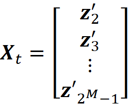
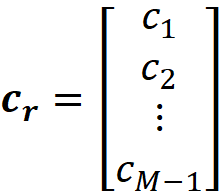
And let Xᵣ be a (2ᴹ-2)×(M-1) matrix defined as:

Here *,i means the i-th column of Xₜ. So Xᵣ is formed by subtracting the last column of Xₜ from the first M-1 columns. We also define the column vector cᵣ as:
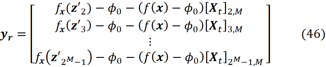
and define the column vector yᵣ with 2ᴹ-2 elements as:
where x is the feature vector that should be explained. Finally, we define the (2ᴹ-2)× (2ᴹ-2) diagonal matrix Wᵣ as:

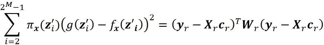
Please note that Wᵣ has no infinite diagonal elements now. It can be shown (the details are given in the appendix) the objective function in Equation 45 can be written as:
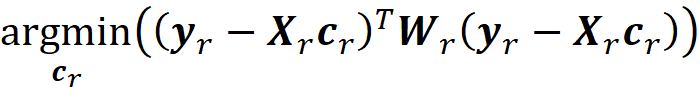
So, we need to solve this minimization problem:
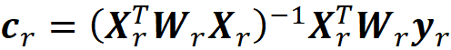
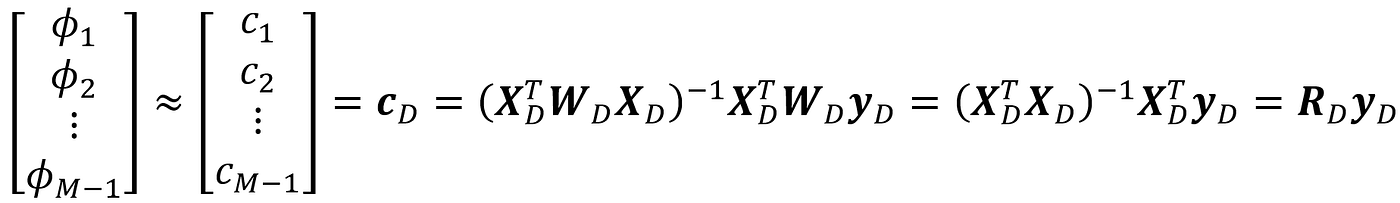
and the value of cᵣ that minimizes this objective function is:
So based on theorem 1 we have:
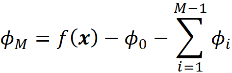
We know that
And once we have ϕ₁ to ϕ_M-1, we can calculate ϕ_M using Equation 22:
So, using this method we can calculate all the SHAP values without dealing with the infinite elements of W. Similar to Equation 41, the term Rᵣ does not depend on a specific data instance to be explained, so if we want to explain multiple data instances, we only need to calculate it once. To implement kernel SHAP using Equation 47, we need to change some of the Python functions. The function generate_coalition_vectors2() in Listing 15 is similar to the one defined in Listing 8, but it doesn’t generate the all-zeros and all-ones coalitions. So it only generates the rows of the matrix Xₜ.
The function generate_pi_values2() is similar to the function generate_pi_values() defined in Listing 10, but it has no exception handling since we have no infinite values of πₓ(z’ᵢ). This function returns the list of the diagonal elements of the matrix diagonal matrix Wᵣ.
The function kernel_shap2() calculates the SHAP values by calling the function calculate_shap_values2(). It calculates ϕ₁ to ϕ_M-1 using Equation 47 and then calculates ϕ_M using them.
We can try kernel_shap2() on our previous model and data set defined in Listing 13.
# Listing 18shap_values = kernel_shap2(rf_model.predict, X_train, weights,
   data_to_explain)
shap_values
Output:
(22.74244968353333,
 array([[ 4.05579906e-02, -4.91062100e-02, -4.69741717e-01,
          9.28299916e-02, -8.88366357e-01, -2.86693056e+00,
          2.19117328e-01, -3.57934593e-02,  4.44089210e-16]]))
As you see the returned SHAP values are almost identical to those of kernel_shap() in Listing 14.
Kernel SHAP with sampling
When a model has so many features, computing the right-hand side of Equation 41 or Equation 47 is still computationally expensive. In that case, we can use a sample of the coalition vectors z’ᵢ to form the coalition matrix X. The coalition matrix X has 2ᴹ rows, and each row is a coalition vector z’ᵢ. The Shapley kernel weight, πₓ(z’ᵢ), gives the weight of the coalition vector z’ᵢ. However, the majority of the coalition vectors have a very small Shapley kernel which means that they don’t contribute that much to the Shapley values. Hence we can ignore those coalition vectors and approximate the Shapely values without them.
If we assume that the Shapley kernel weights give the probability distribution of the coalition vectors, we can sample (with replacement) a subset of D coalition vectors from the original 2ᴹ-2 coalition vectors that don’t include z’₁ and z’_2ᴹ. We place these vectors in the D×M coalition matrix X_p:
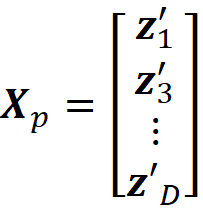
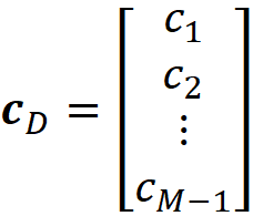
where z’₁... z’ᴅ are the sampled coalition vectors. Now we can use Equation 47 to calculate the Shapley values using this new coalition matrix. We form the D×(M-1) matrix Xᴅ as:

the column vector cᴅ is defined as:
and we define the column vector yᴅ with D elements as:
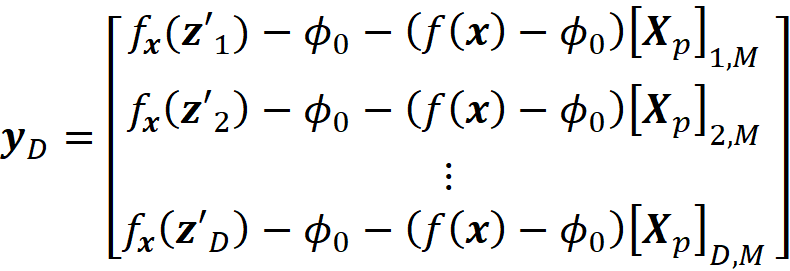
Finally, we define the D×D diagonal matrix Wᴅ as:

The reason that all the Shapley kernel weights are 1 is that we already sampled the coalition vectors using their Shapley kernel weights. So the sampled coalitions have are now weighted equally in the new coalition matrix. Now we can use Equation 47 to calculate Shapley values using the sampled coalition vectors:
Now we can use a modified version of Equation 47 to calculate Shapley values using the sampled coalition vectors. To implement this method in Python, we only need to modify the functions defined in Listing 17:
In kernel_shap3(), we use the function choice() in Numpy to sample the coalition vectors using their normalized Shaply kernel weights. Here we sample half of the original coalition vectors (but it can be a different number). The sampled coalition vectors will be passed to calculate_shap_values3() to calculate the SHAP values. This time we don’t need the πₓ(z’ᵢ) values since they are all equal to 1.
Kernel SHAP in the SHAP library
The class kernelExplainer() can be used to calculate the SHAP values using the kernel SHAP method. We use the same data set and model defined in Listing 13. This class takes the model and training data set and its method shap_values() returns ϕ₁ to ϕ_M. The value of ϕ₀ is stored in the field expected_value.
explainer = shap.KernelExplainer(rf_model.predict, X_train)
k_shap_values = explainer.shap_values(data_to_explain)
phi0 = explainer.expected_value
k_shap_values### Output:
array([[ 0.04055799, -0.04910621, -0.46974172,  0.09282999, -0.88836636, -2.86693056,  0.21911733, -0.03579346,  0. ]])
phi0### Output:
22.742449683533327
As you see the output is almost equal to that of kernel_shap() in Listing 14 or kernel_shap2() in Listing 18. Unlike the class Explainer, KernelExplainer doesn’t sample from the training data set automatically and will use the whole training data set passed to it. We can either manually sample the data set like the example above or use the methods shap.sample() and shap.kmeans() to do that. For example, we can randomly sample 100 rows of the training data set using shap.sample():
explainer = shap.KernelExplainer(rf_model.predict, shap.sample(X,
   100))
Or we can summarize the training data set using shap.kmeans():
explainer = shap.KernelExplainer(rf_model.predict, shap.kmeans(X,
   100))
Here the k-means algorithm is used to find 100 clusters in the training data set, and the weight of each cluster is proportional to the number of data points in it. The result is the mean of 100 clusters with their corresponding weights. Now this weighted data set is used as a sample of the original data set to calculate the SHAP values. The following code shows how k-means sampling can be implemented in Python. We first use the class KMeans in the scikit-learn library to divide X into 100 clusters. Then the weights array is created based on the number of data points on each cluster. Finally, the center of the clusters and the weights array are passed to kernel_shap2() to generate the SHAP values.
kmeans = KMeans(n_clusters=100, random_state=10).fit(X)cluster_size = np.bincount(kmeans.labels_)
weights = cluster_size / np.sum(cluster_size)
X_train_kmeans = kmeans.cluster_centers_
shap_values = kernel_shap2(rf_model.predict, X_train_kmeans,
   weights, data_to_explain)
SHAP values of tree-based models
Remember that we used this equation:
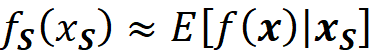
to calculate the SHAP values (refer to Equation 23). To calculate the conditional expectation in the above equation, we used the approximation given in Equation 29:

As we see in this section, for tree-based models (trees and ensembles of trees), there is a better way to calculate E[f(x)|xₛ].
As we mentioned before SHAP is a model-agnostic explainer, so the model to be explained is a black box, and we don’t know its type. But, in methods like linear SHAP or tree SHAP, we should know the type of the model, so these methods are not truly model-agnostic. However, this is not an important limitation, since, in real-world applications, we usually know the type of model to be explained.
Let’s start by trying a tree-based model on the Boston data set.
# Listing 20d = load_boston()
df = pd.DataFrame(d['data'], columns=d['feature_names'])
y = pd.Series(d['target'])
X = df[['AGE', 'RAD', 'TAX', 'DIS']]

tree_model = DecisionTreeRegressor(max_depth=3)
tree_model.fit(X, y)fig = plt.figure(figsize=(20, 10))
plot_tree(tree_model, feature_names=X.columns, fontsize =16)
plt.show()
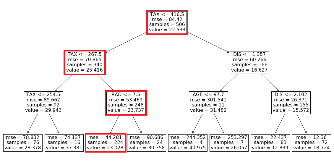
Here we use a decision tree regressor (from the scikit-learn library) to model a subset of the Boston data set with 4 features (AGE, RAD, TAX, and DIS). We fit the model and plot the resulting tree which is shown in Figure 9.
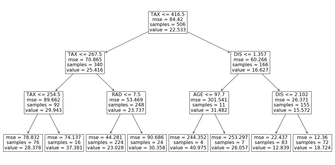
Each internal node in this tree is labeled with a feature of the data set and represents a test on that feature. Each branch of that node represents the outcome of the test. The value of each leaf node gives the prediction of the tree model for a feature vector that passes all the tests in the path from the root of the tree to the leaf. For example, we can use this model to predict the target value of the first row of X in Listing 20:
X.iloc[0]### Output:
AGE     65.20
RAD      1.00
TAX    296.00
DIS      4.09
tree_model.predict(X.iloc[0:1])### Output:
array([23.02767857])
For this row, we have TAX <=416.5, TAX <= 267.5, and RID <= 7.5, so starting from the root of the tree, we end up in a leaf with a value of 23.028 (Figure 10). This value is the model prediction for the first row of X.
Now let’s see what happens if we have an NA value in the feature vector. Suppose that we don’t have the values of DIS in the first row of X. So the feature vector is:

Based on these values we can go from the root to the internal node with the test RAD<=7.5 (Figure 11), but we cannot go further since we don’t have the value of RAD. However, by looking at the left and right leaves we know that in this model we only have two possible predictions for this feature vector. If RAD<=7.5, then the prediction is 23.028. Otherwise, the prediction is 30.358. We also know how many data samples of the training data set fell in each leaf. Here 224 out of 248 samples fell in the left leaf and the remaining 24 samples fell in the right leaf (Figure 11). The number of samples that fall in each node is called the cover of that node, so the cover of the node with the test RAD<=7.5 is 248. Based on these results, we can say that the probability of getting the value of the left node is 224/248 and the probability of getting the value of the right node is 24/248. Hence the predicted value of the model for this feature vector is:

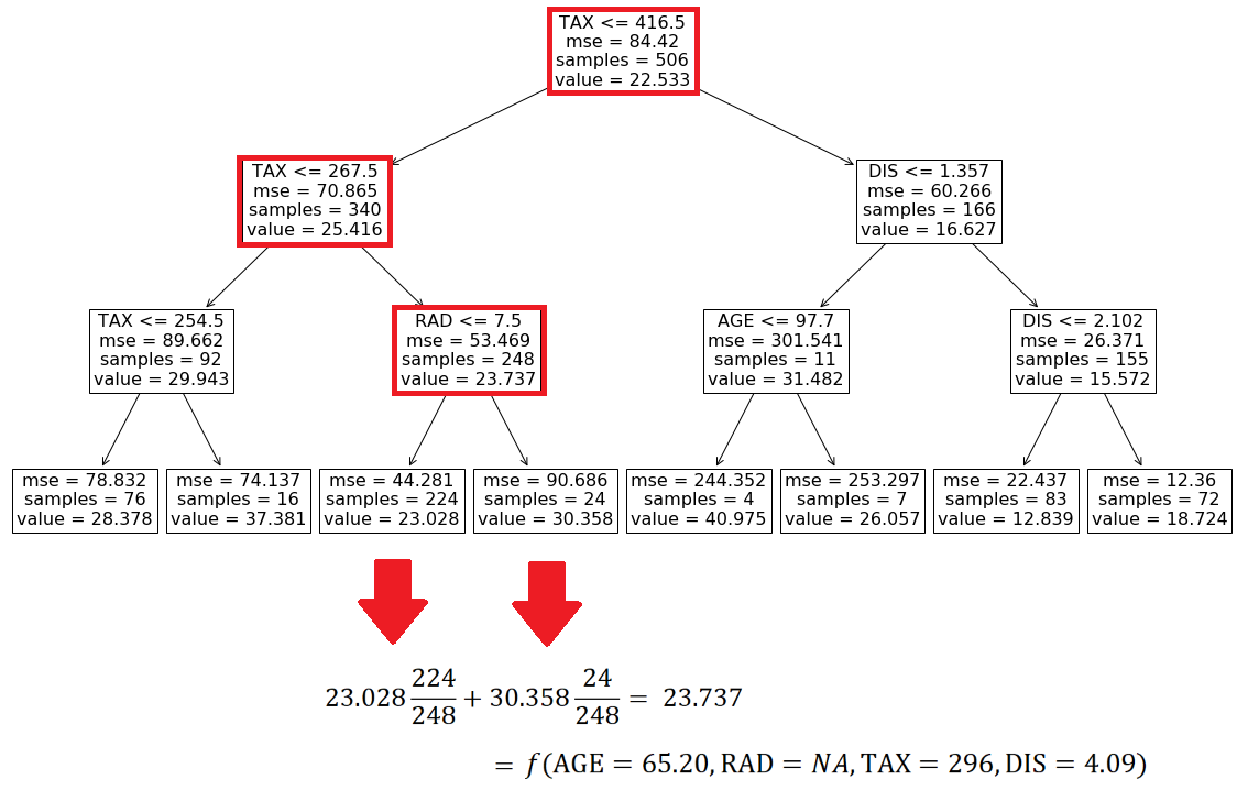
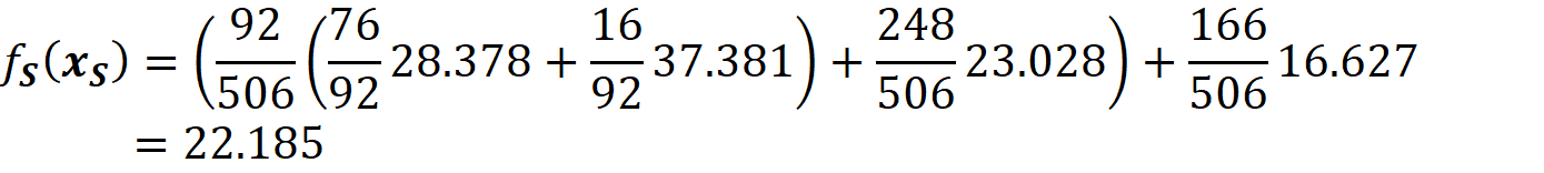
This is the average of the values of the left and right leaves weighted by their covers. If you look at Figure 11, you will notice that the value of the node which tests RAD <=7.5 is the same number (23.737). Here, scikit-learn calculates and shows these average values for all the internal nodes of the tree. Let’s see another example. Here the feature vector is:

At the root node, we don’t know the value of TAX, so we take the weighted average of the left and right branches. In the right branch, we don’t have the value of the features tested on any internal nodes, so we take the weighted average of the values of all leaves:

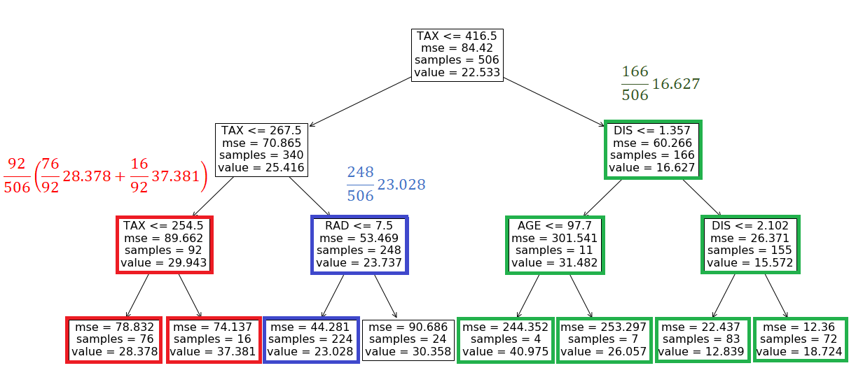
The probability of getting this value is 166/506. In the left branch of the root, we don’t have the value of TAX, so we take the weighted average of the values of the nodes with tests TAX<=254.5 and RAD<=7.5. For the node that tests TAX<=254.5, we take the weighted average of both leaves. We know the value of RAD, so for the node that tests RAD<=7.5, the value is 23.028 with a probability of 248/506. Finally, the prediction of the model for this feature vector is (Figure 12):
Now that we know how to handle the NA features in a tree-based model, we can use the recursive algorithm in Algorithm 1 to calculate fₛ(xₛ)=E[f(x)|xₛ].
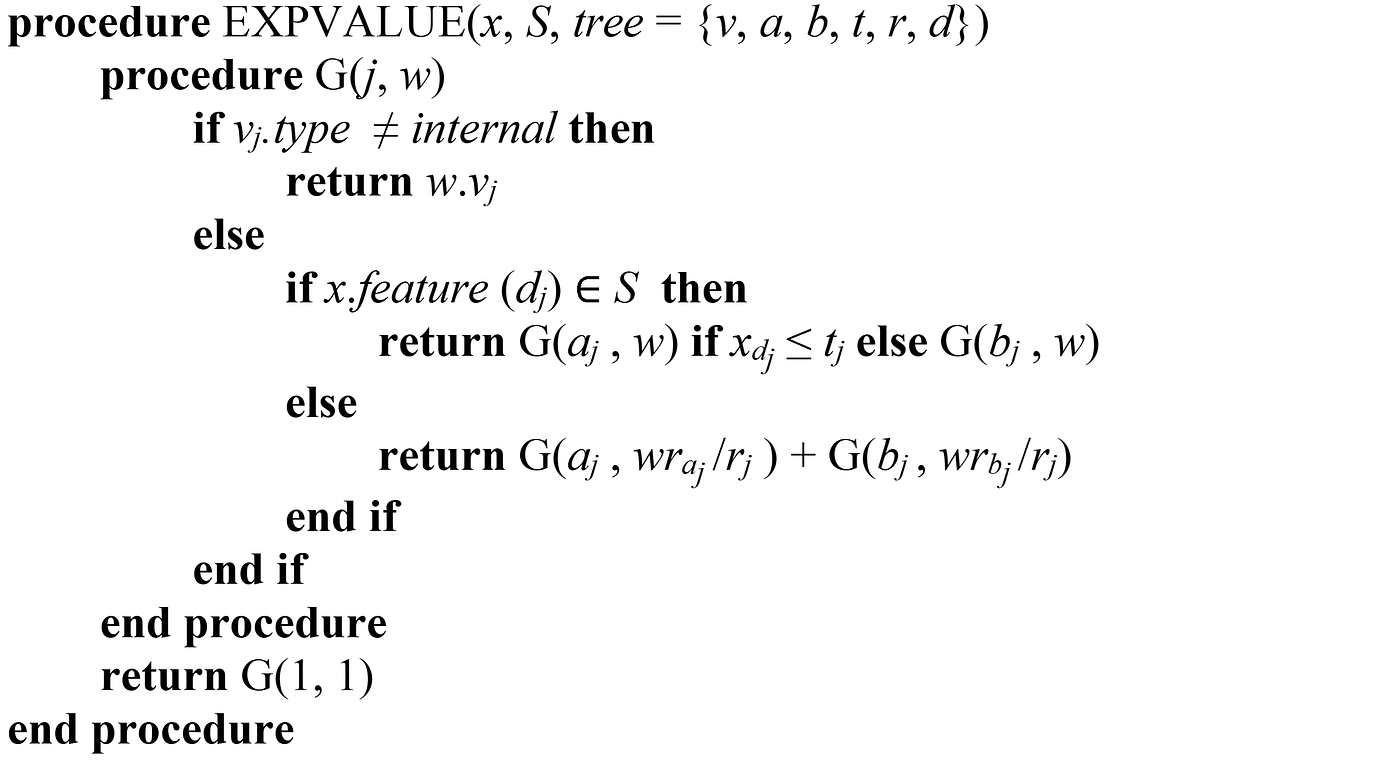
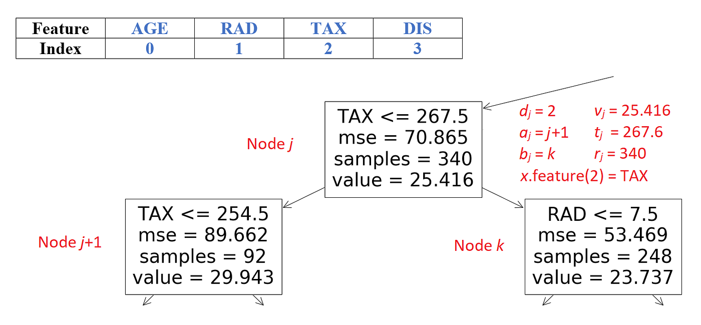
The function EXPVALUE() takes the feature vector to be explained (x), the coalition S (that contains the available features), and the tree model, and calculates fₛ(xₛ)≈E[f(x)|xₛ]. In the tree model, each node has an index, and the index of the root is 1. v is a vector of node values. vⱼ.type indicates if a node is an internal node or a leaf. The vectors a and b represent the left and right node indexes for each internal node. The vector t contains the threshold for each internal node and d is a vector of indexes of the features used for splitting in internal nodes. The vector r contains the cover of each node. x.feature(dⱼ) gives the name of the feature in x whose index is dⱼ. Figure 13 shows the value of these vectors for a sample node.
The function G() takes the index of a node and an accumulator. For an internal node, if its feature is not a member of S (which means that we don’t have the value of that feature), the function recursively calculates the value of the left and right branches and returns the weighted average of them.
If the feature of the node is in S, then the left or right branch is chosen by comparing the value of that feature with the threshold, and the value of the branch is calculated recursively. Finally, for a leaf node, its value is multiplied by the cover of the leaf and returned. The Python implementation of this algorithm is given in Listing 21.
We can test this function on the coalition shown in Figure 11 and Figure 12:
expvalue(tree_model, x=X[:1].T.squeeze(), S=['TAX', 'AGE', 'DIS'])### Output:
23.73709677419353
expvalue(tree_model, x=X[:1].T.squeeze(), S=['RAD'])### Output:
22.18510728402032
What happens if we try an empty list for S?
expvalue(tree_model, x=X[:1].T.squeeze(), S=[])### Output:
22.532806324110666
This is the weighted average of the value of all the leaves in the tree. In fact, scikit-learn has already calculated it as the value of the root node (look at Figure 9). This is equal to the average of the predictions of all the data instances in the training data set. That is because, for each data instance, the model prediction is simply the value of one of the leaves, and we know the weight of each value for the whole training data set. From Equation 7, when we have no available features, the model prediction is the average of the predictions for the instances in a sample of the training data set, and here we use the whole training data set instead of a sample. We also know from property 1 that ϕ₀ =E[f(x)]. So running expvalue() with an empty coalition returns ϕ₀. In addition, the value of the root node calculated by the scikit-learn is also equal to ϕ₀.
Now we can use this function to calculate the SHAP value of a decision tree regressor. We can use the same code in Listing 5 with some minor modifications. In function coalition_contribution() we use expvalue() to calculate the model prediction for each coalition, and in calculate_exact_tree_shap_values() we use the value of the root node as ϕ₀.
We can now test this function to explain a row of X:
# Listing 23calculate_exact_tree_shap_values(tree_model, X.iloc[470])
Output:
(22.532806324110698,
 [[0.17363555010556078,
   1.6225955204216118,
   -6.753886031609969,
   1.1484597480832428]])
The function EXPVALUE() defined in Algorithm 1 is a much better choice to calculate fₛ(xₛ). Now we have:

This allows us to get the exact value of fₛ(xₛ) for a tree-based model trained on a certain data set, and the answer is more reliable than the approximation given in
Remember that we used this approximation to calculate the SHAP values using exact and kernel SHAP methods.
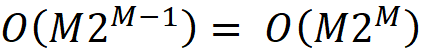
The time complexity of Algorithm 1 is proportional to the number of leaves in the tree. That is because the worst-case scenario is when we have a coalition that doesn’t contain any of the features of the internal nodes of the tree. In that case, the algorithm needs to calculate the weighted average of the values of all the leaves. So the time complicity of EXVALUE() is O(L) where L is the number leaves. We have M features, and for each feature, we must evaluate 2ᴹ-1 coalitions (excluding that feature). So, the time complexity of finding the SHAP values of all the features is O(LM2ᴹ⁻¹)=O(LM2ᴹ)
Finally, for an ensemble model, we can use T trees in an ensemble which leads to a time complexity of O(TLM2ᴹ) for computing the SHAP values of all M features. As a result, computing the SHAP values of a tree-based model using Algorithm 1 is computationally expensive for large values of M.
Tree SHAP algorithm
Lundberg et. al [3] proposed an efficient algorithm that can reduce the time complexity of finding the SAHP values of a tree-based model. Unfortunately, the algorithm given in [3] has so many typos and is not explained clearly. So, in this section, I will present a corrected version of this algorithm and try to explain how it works. Algorithm 2 gives a corrected version of the original algorithm in [3] (the corrections are marked in red).
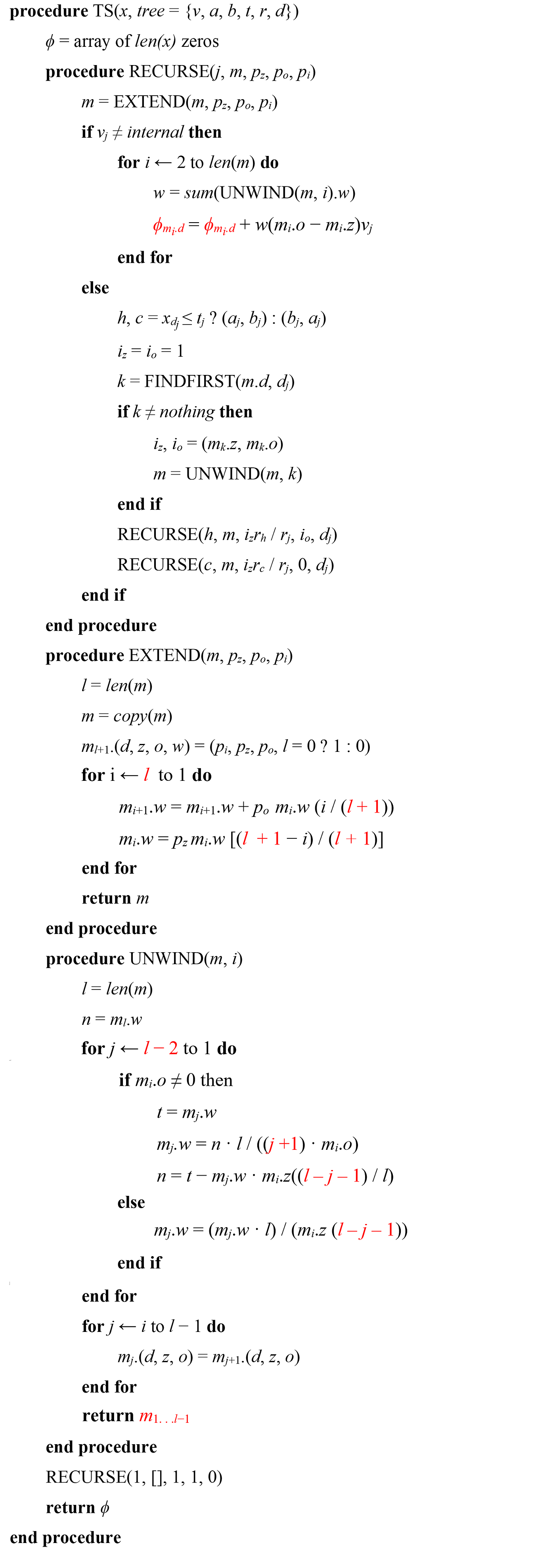
The Python implementation of this algorithm is given in Listing 24 (since in Python the arrays and dataframes are zero-indexed, some modifications are needed).
We can test the tree_shap() function with the same row that was used in Listing 23:
# Listing 25
tree_shap(tree_model, X.iloc[470])
Output:
(22.532806324110698,
 array([ 0.17363555,  1.62259552, -6.75388603,  1.14845975]))
Here we get the same SHAP values as Listing 23.
How does the tree SHAP algorithm work? (optional)
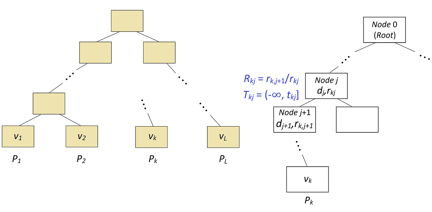
To understand this algorithm, we first need to understand the math behind it [4]. Here we use the same notation of Algorithm 1, but we also need to introduce some additional notations (Figure 14). Suppose that we have a tree with L leaves, and the values of these leaves are v₁…v_L. A path Pₖ is defined as the set of internal nodes starting from the root and ending at the leaf with the value of vₖ (We only include the internal nodes, so the leaf itself is not included in the path). Hence, we have L paths in this tree (P₁…P_L).
Let j be the j-th internal node in path Pₖ (so for each path Pₖ, j is zero for the root node and increases by 1 for the next node in the path), and let Dₖ = {dⱼ | j ϵ Pₖ} be the set of the indices of unique features used for splitting in internal nodes in path Pₖ (here we assume that each feature in the feature vector x has an index). In addition, tₖⱼ denotes the threshold of the internal node j in path Pₖ. Hence {tₖⱼ | j ϵ Pₖ} is the set of the thresholds of the internal nodes in path Pₖ. We assume that Tₖⱼ = (-∞, tₖⱼ] if node j connects to its left child in path Pₖ and Tₖⱼ = (tₖⱼ, ∞) if node j connects to its right child in path Pₖ. Finally, the covering ratios along the path Pₖ are denoted by the set {Rₖⱼ | j ϵ Pₖ} where Rₖⱼ = r_(k,j+1)/rₖⱼ and rₖⱼ is the cover of the internal node j in path Pₖ.
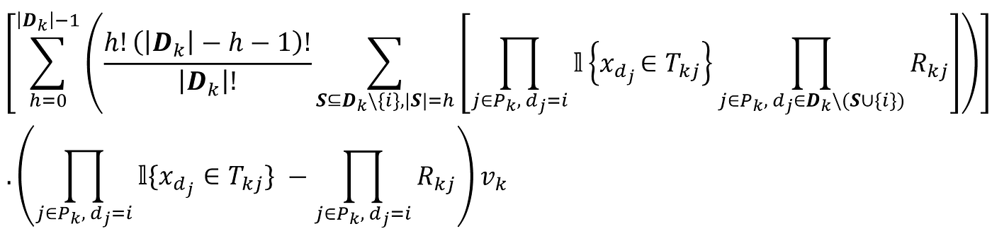
Now it can be shown that the value ϕᵢ can be calculated using the following formula:
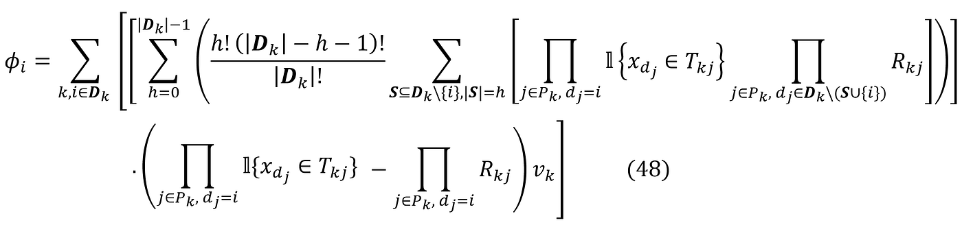
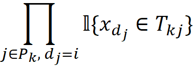
where 𝟙{.} is the indicator function, so

The proof of this equation is given in [4].
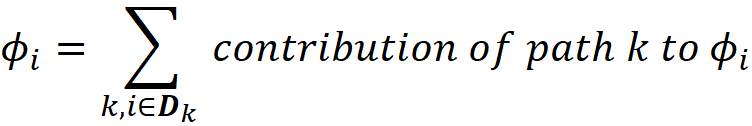
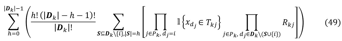
The first sum in Equation 48 is over all the paths in which a node contains feature i. As mentioned before, Dₖ is the set of all the unique features in path Pₖ. The third sum in this equation is over all the coalitions of Dₖ with m elements that don’t contain the feature i. So, for each feature i, we need to find the paths that contain this feature and calculate the contribution of each path to the SHAP value of that feature. Based on Equation 48, the SHAP value is then the sum of all these contributions:
Now let’s see how the tree SHAP algorithm works. Algorithm 2 recursively finds all the paths in a tree. At the end of each path, it calculates the contribution of that path to all the features and adds them to the variable ϕᵢ (so each ϕᵢ in algorithm 2 is an accumulator for the SHAP value of feature i). When the algorithm covers all the paths, ϕᵢ is equal to the SHAP value of feature i. The variable m in Algorithm 2 (which is equivalent to the dataframe m in Listing 24) is a table with 4 fields: d, z, o, and w. These fields keep the information that we need in each path to calculate its contribution to the SHAP value of feature i. When the algorithm is traveling a path, m contains the indices of all the unique features found in that path so far. These indices are stored in the field d in m. In function RECURSE() if we find a leaf, then we use this loop:

Here w = sum(UNWIND(m, i).w) is equal to:
mᵢ.o in table m gives the value of:
And mᵢ.z gives:

So calculating w(mᵢ.o-mᵢ.z).vⱼ is equivalent to calculating:
in Equation 48. Hence, the For loop calculates the contribution of the path to the SHAP value of the features that are present in that path. The For loop starts from 2 since we start filling m at that index. The function RECURSE(j, m, pz , po, pᵢ) takes five parameters. j is the index of the current node in the tree (we initialize it with 0 which is the index of the root node). The index of the feature which is used to split the previous node along the path is stored in pᵢ. The feature which is used to split the current node is vⱼ. Based on the value of this feature, the left or right child node should be chosen. The index of the chosen node is called the hot index (h), and the index of the other child node will be the cold index (c):

Since we only need the set of unique features in a path, the algorithm checks if vⱼ is already stored in m or not? If it is a duplicate feature, it will be removed using UNWIND(). The function RECURSE() calls itself at the end for both the hot index and cold index:
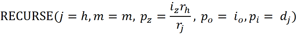
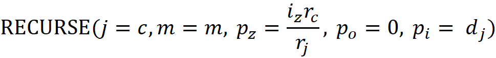
If dⱼ is a duplicate feature, its covering ratio in m (the field mₖ.z) is found and stored in iz. Otherwise, we have iz=1. The covering ratio of the current node (which is either rₕ/rⱼor r𝒸/rⱼ) is then multiplied with i𝓏 and passed as p𝓏 to RECURSE(). Hence, p𝓏 accumulates
along the path. pₒ keeps the track of
For a hot index, we pass mₖ.o (if dⱼ is a duplicate feature) or 1 as pₒ to RECURSE() and for a cold index, we pass 0 as pₒ. The function EXTEND() is called to store the information for each feature found along the path. It stores pᵢ, pz, and pₒ in mᵢ.d, mᵢ.z, and mᵢ.o respectively. It also calculates
And stores it in mᵢ.w.
But how these values are generated along a path? The function EXTEND() is responsible for generating the values of
for h=0, 1, …,|Dₖ|. At the leaf node, the field w in m contains the values of Equation 50 for h=0, 1, …,|Dₖ|. Please note that in Equation 48 the third sum is over S⊆Dₖ\{i},|S|=h. So the calculate the contribution of the path to SHAP values, first we need to remove the feature {i} from Equation 50. That is why we first call UNWIND(m, i).w) and then apply SUM() to the result. As mentioned before sum(UNWIND(m, i).w) is equal to Equation 49. Please also note that both EXTEND() and UNWIND() make a copy of m before changing and returning it. The copied m will be used for the current node while the original m remains intact for the previous node. As a result, as we travel along the tree, m only contains the set of unique features along the current path.
Algorithm 2 reduces the time complexity of Algorithm 1 from exponential to low order polynomial. The loops in functions EXTEND() and UNWIND() are all bounded by the length of m. Since m keeps the track of the unique features along a path, it is bounded by D, the maximum depth of a tree. Hence, the time complexity of UNWIND() and EXTEND() is O(D). The loop in function RECURSE() is also bounded by the length of m. However, for a leaf, the function UNWIND() is called inside that loop, so the time complexity of RECURSE() is O(D²) since UNWIND() is nested inside a loop bounded by D. The function RECURSE() should find all the paths of the tree, and the number of paths is equal to the number of leaves. So assuming that L is the maximum number of leaves in any tree, the time complexity of RECURSE() for the whole tree will be O(LD²). Finally, for an ensemble of T trees, the time complexity becomes O(TLD²).
Tree SHAP for tree ensembles
We can easily use the tree_shap() function to calculate the SHAP values of tree ensemble models. Suppose that we have an ensemble of T trees. We can calculate the SHAP values of each tree separately, and we call the SHAP value of feature i in the j-th tree ϕᵢ⁽ʲ⁾. Since all these trees are equally important, the SHAP value of the feature i for the entire ensemble is simply the average of the SHAP values of i for all the trees inside the ensemble:
The function tree_shap_ensemble() in Listing 26 can be used to calculate the SHAP values of a tree ensemble model.
This function uses the tree SHAP algorithm to calculate the SHAP values of each tree in the ensemble and then takes the average of these values. We can now test this function on a random forest model:
# Listing 27d = load_boston()
df = pd.DataFrame(d['data'], columns=d['feature_names'])
y = pd.Series(d['target'])
X = df[['AGE', 'RAD', 'TAX', 'DIS']]

rf_model2 = RandomForestRegressor(random_state=0, n_estimators=4).fit(X, y)
tree_shap_ensemble(rf_model2, X.iloc[470])### Output:
(22.340563241106732,
 array([-0.60018849,  1.36914776, -6.2207912 ,  2.33626868]))
Tree SHAP in the SHAP library
The class TreeExplainer in the SHAP library can be used to calculate the SHAP values using the tree SHAP method for both trees and tree ensembles. Here we use this class to calculate the SHAP values of the data set and model defined in Listing 20.
explainer = shap.TreeExplainer(tree_model)
shap_values = explainer.shap_values(X.iloc[470])
shap_values### Output:
array([ 0.17363555,  1.62259552, -6.75388603,  1.14845975])
explainer.expected_value### Output:
array([22.53280632])
As you see the SHAP values are almost the same as the SHAP values returned by calculate_shap_values() in Listing 23 and tree_shap() in Listing 25. This class can be also used for the random forest defined in Listing 27 and the output is almost the same as the output of that Listing.
explainer = shap.TreeExplainer(rf_model2)
shap_values = explainer.shap_values(X.iloc[470])
shap_values### Output:
array([-0.60018849,  1.36914776, -6.2207912 ,  2.33626868])
explainer.expected_value### Output:
array([22.34056324])
SHAP Plots
Shap library has some nice tools to visualize the SHAP values. Waterfall plots can display the SHAP values for individual feature vectors. As an example, we train an XGBoost model on the Boston data set and display the waterfall plot for one instance of X:
d = load_boston()
df = pd.DataFrame(d['data'], columns=d['feature_names'])
X = df
y = pd.Series(d['target'])xgb_model = xgboost.XGBRegressor(random_state=1).fit(X, y)explainer = shap.Explainer(xgb_model, X)
explanation_object = explainer(X)
shap_values = explainer.shap_values(X)# visualize the first prediction's explanation
shap.plots.waterfall(explanation_object[0])
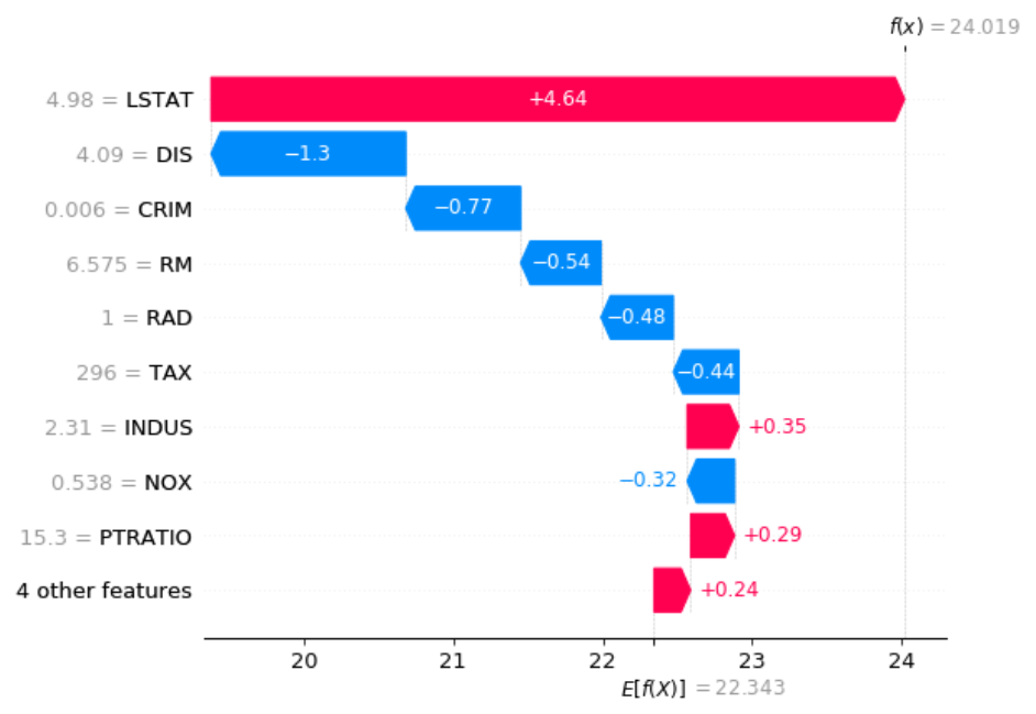
Remember that from Equation 22, we have:
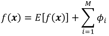
A waterfall plot can visualize this equation for us. The bottom of a waterfall plot starts at E[f(x)]=22.343, and each arrow in this plot shows the positive (red) or negative (blue) contribution of each feature to the prediction. The length of each arrow is equal to the absolute SHAP value of its corresponding feature. The SHAP value is written over the arrow, and the value of the corresponding feature is also written on the vertical axis (for example in the plot above, the value of the feature LSTAT is 4.98, and its SHAP value is 4.64). If the SHAP value is positive, the arrow is red and goes to the right. For a negative SHAP value, it is blue and goes to the left. By following these arrows, we finally reach the value of the model prediction f(x)=21.019. The features are sorted by the absolute of their SHAP values, so the feature with the greatest absolute SHAP value sits on top. Please note that we need to directly pass the Explainer object to waterfall() not the SHAP values returned by shap_values() method of Explainer.
We can also use a force plot to visualize the SHAP values:
shap.initjs()
shap.plots.force(explanation_object[0])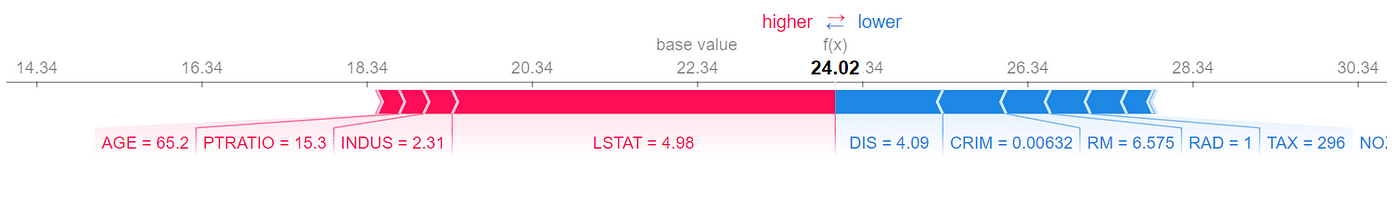
A force plot is like a waterfall plot, however, the arrows are stacked horizontally. The red and arrows are sorted based on their length, so the red arrows get longer from left to right and the blue arrows get longer from right to left. The value of each feature (not its SHAP value) is written behind its corresponding arrow. The longest red and blues arrows intersect at f(x)=21.019. The value of E[f(x)]=22.343 is also shown in the plot labeled as the base value.
We can also use a bar plot to display the SHAP values. We can use the function shap.plots.bar() which takes an Explanation object. The bar plot doesn’t show the arrows, the values of f(x) and E[f(x)], and the value of the features. The length of each bar is equal to the absolute SHAP value of its corresponding feature. The bar is colored red/blue for positive/negative SHAP values, and the SHAP values are written beside each bar. The features are sorted by the absolute of their SHAP values.
shap.plots.bar(explanation_object[0])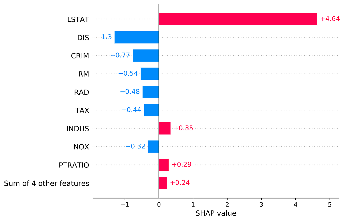
We can also force the bar plot to only show the absolute SHAP values:
shap.plots.bar(explanation_object[0].abs)
A beeswarm plot is useful to summarize the SHAP analysis for lots of instances. First, we use it just for one instance. The function shap.plots.beeswarm() takes an Explanation object. Please note that the function has a bug, and when you call it, it changes the SHAP values of theExplanation object that it takes, so you should always pass a deep copy of the Explanation object to it.
import copy
shap.plots.beeswarm(copy.deepcopy(explanation_object[0:1]))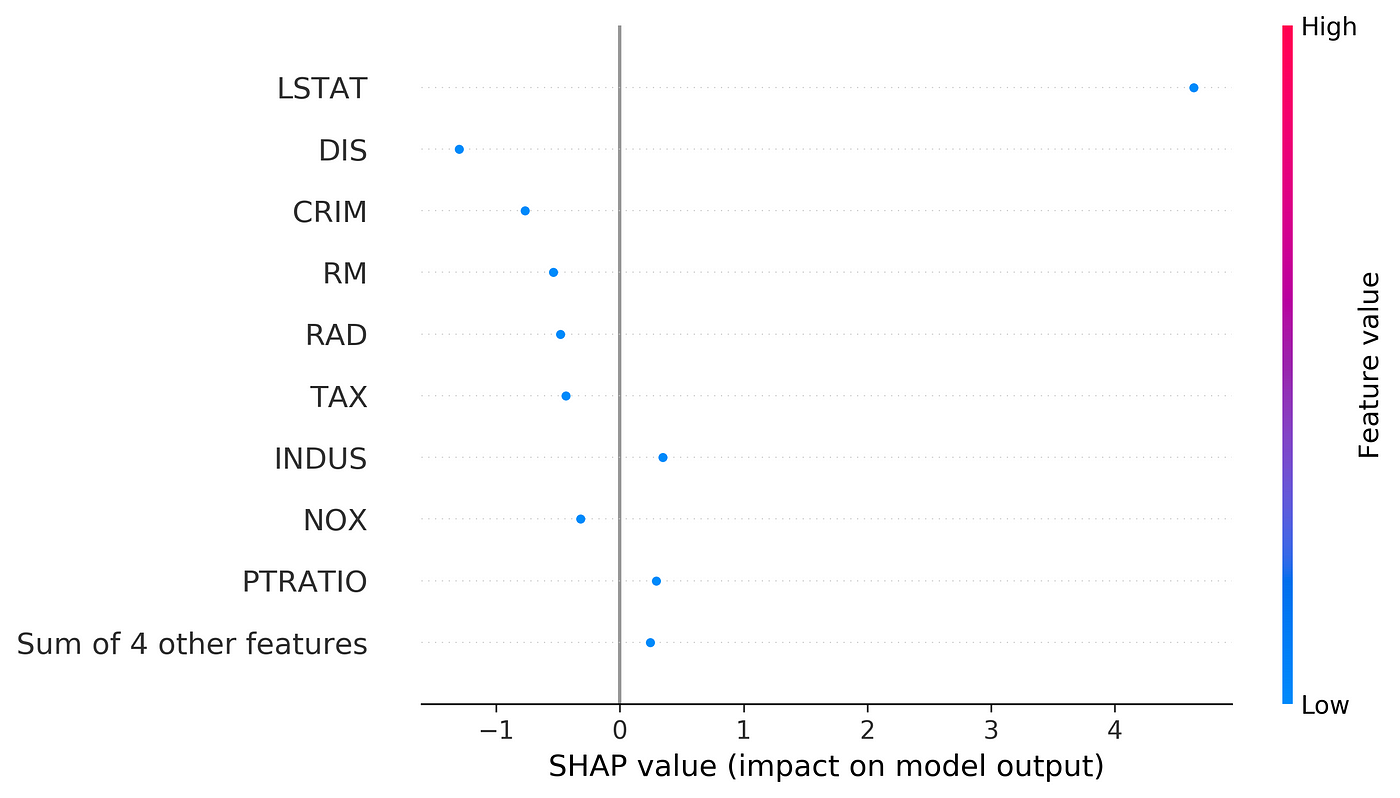
The plot is similar to a bar plot, however, instead of the bar we have dots for each SHAP value. The x position of each dot gives the SHAP value of the corresponding feature. Since we only have one instance all the dots have the same color. Now we try it for two instances. Now for each feature, we have two dotes, and each dot represents one of the instances.
shap.plots.beeswarm(copy.deepcopy(explanation_object[0:2]))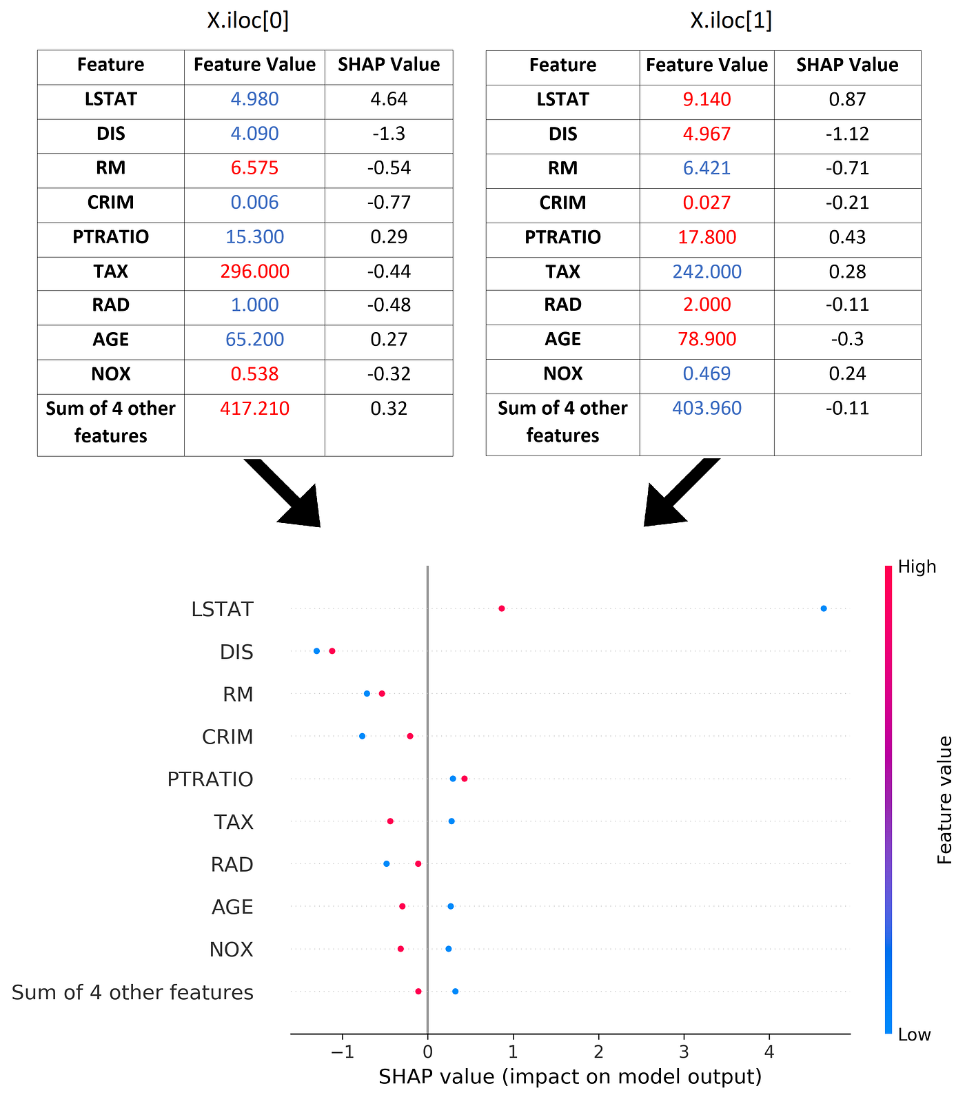
The dots are colored based on the value of the corresponding feature. For each feature, the instance that has a higher value (of that feature) is red and the other one is blue. But how the features are sorted when we have more than one instance? The features are sorted based on the average of the absolute SHAP values of all instances. Now we can try it on more instances:
shap.plots.beeswarm(copy.deepcopy(explanation_object))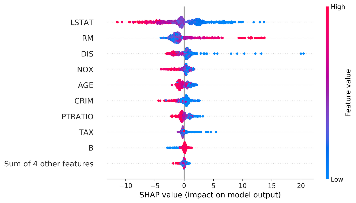
As you in this plot, the maximum SHAP value belongs to the feature DIS, but LSTAT has the highest average for all the instances. We can change this and sort the feature by their maximum absolute SHAP value.
shap.plots.beeswarm(copy.deepcopy(explanation_object),
   order=explanation_object.abs.max(0))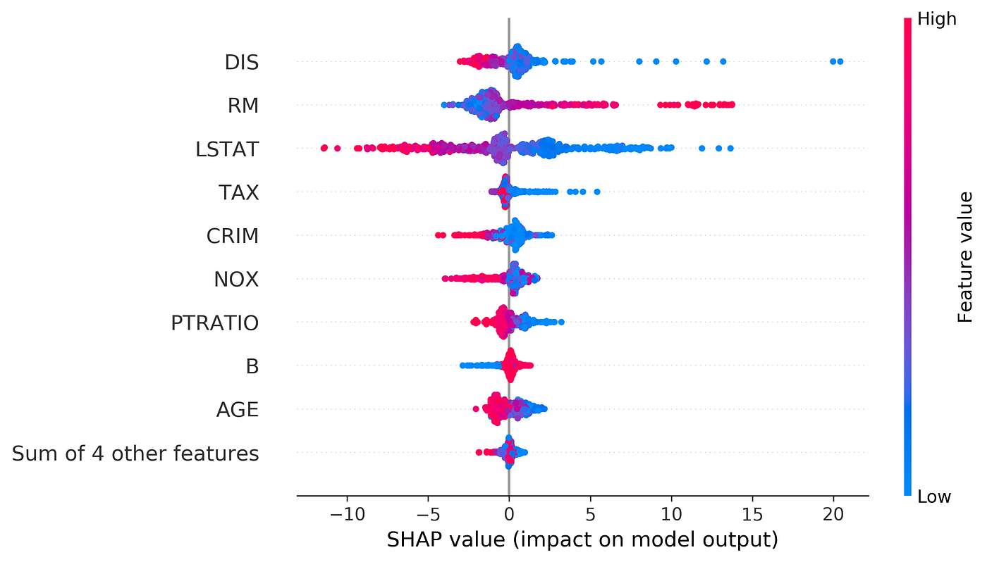
Now DIS sits on top. We can also use more than one instance with a bar plot. In that case, it will calculate the average of the absolute SHAP value of all instances and sort the features based on that. The average of the absolute SHAP values is also shown beside the bars.
shap.plots.bar(explanation_object)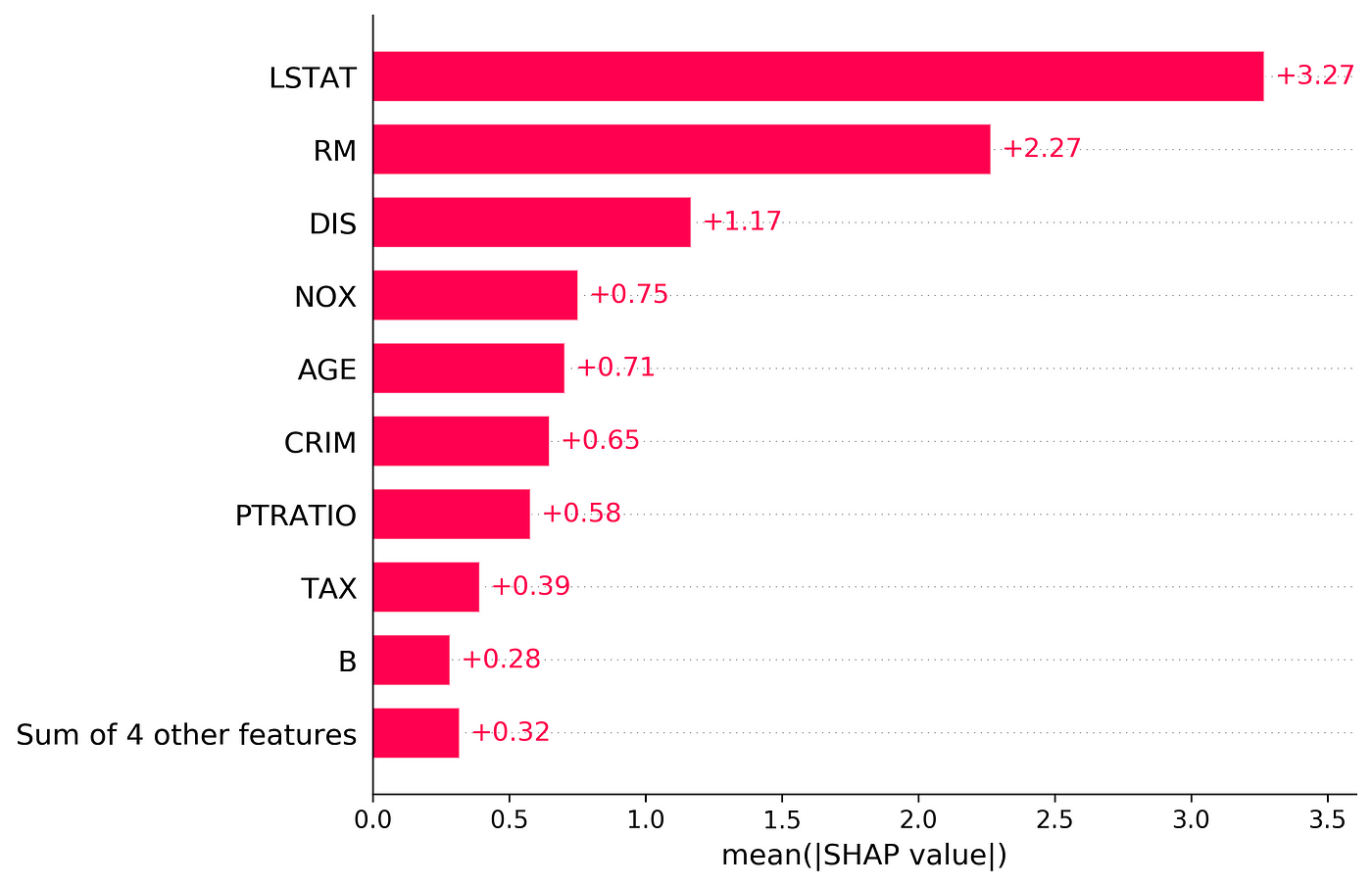
Finally, we can display a force plot for multiple instances. Here is an example for 3 instances:
shap.force_plot(explainer.expected_value, shap_values[0:3,:],
   X.iloc[0:3,:], plot_cmap="DrDb")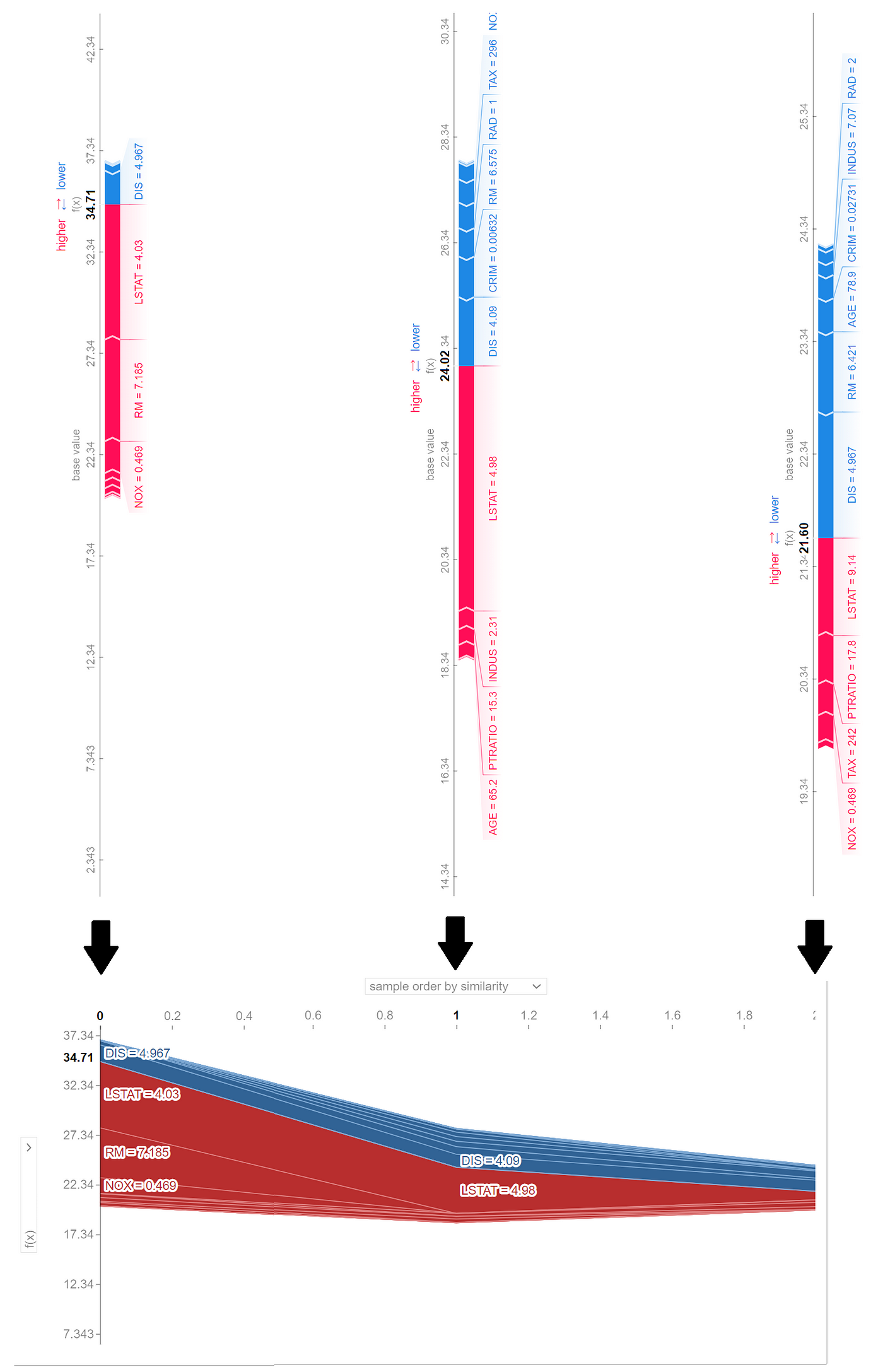
This plot is a combination of 3 individual force plots (like the one in Equation 14) that are rotated 90 degrees and stacked horizontally (refer to Figure 16). Here is another example with more instances:
shap.force_plot(explainer.expected_value, shap_values, X,
    plot_cmap="DrDb")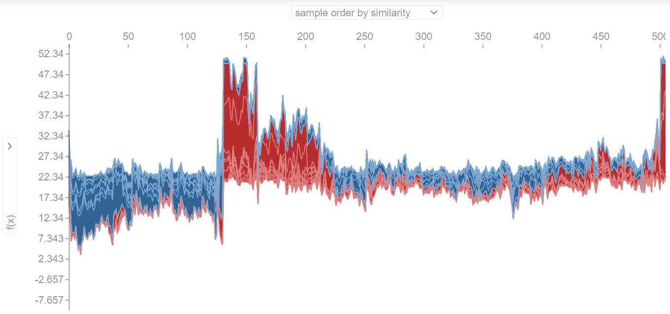
We can choose how the individual force plots are stacked. For example, in Figure 25 the individual plots are stacked based on similarity. If we assume that the SHAP values of each instance form a point in an M-dimensional space, then the similarity is determined by the Euclidian distance between these points, and the points (or instances) that are more similar (have smaller distance) are stacked together. There are some other options to stack the instances. For example, we can sort them based on the value of f(x) for each instance. This is shown in Figure 26. Here the value of f(x) for instances decreases from left to right.
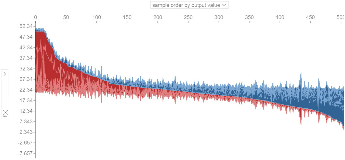
Explaining machine learning models is an important topic. By explaining, we mean that we want to have a qualitative understanding of the relationship between the individual prediction of the model and the features used to generate that prediction. We can explain a complex model using a simple, interpretable model explainer and determine its feature importance. SHAP is an individualized model-agnostic explainer that was developed based on a game-theoretic concept named Shapley values. The SHAP values provide the coefficients of a linear model that can in principle explain any machine learning model.
SHAP values have some desirable theoretical properties, however, in practice, calculating the exact SHAP values is computationally expensive, so we use some methods like kernel SHAP to approximate the SHAP values. In this article, we first explained the mathematical concept of Shapley values and how they can be used to explain machine learning models. We also discussed the SHAP vales and the different algorithms that can be used to estimate them. All these algorithms were implemented in Pythom from scratch. Finally, we discussed the SHAP library in Python and the plotting tools that it provides to visualize the SHAP values.
I hope that you enjoyed reading this article. Please let me know if you have any questions or suggestions. All the Code Listings in this article are available for download as a Jupyter notebook from GitHub at: https://github.com/reza-bagheri/SHAP
References
1-Scott M Lundberg and Su-In Lee. A unified approach to interpreting model predictions. In Proceedings of the 31st international conference on neural information processing systems, pages 4768–4777, 2017.
2- Scott M Lundberg and Su-In Lee. A unified approach to interpreting model predictions. In Proceedings of the 31st international conference on neural information processing systems (2017), Supplementary material (https://papers.nips.cc/paper/2017/file/8a20a8621978632d76c43dfd28b67767-Supplemental.zip).
3-Scott M Lundberg, Gabriel G Erion, and Su-In Lee. Consistent individualized feature attribution for tree ensembles. arXiv preprint arXiv:1802.03888, 2018.
4-Jilei Yang. Fast TreeSHAP: Accelerating SHAP Value Computation for Trees.
arXiv preprint arXiv:2109.09847, 2021.
Appendix
Proof of Linear SHAP equation
Suppose that our predictive model f is a linear regression model:
where x₀=1, and the features Xᵢ, i = 1, …, M are independent. Using Equation 28 we can write:
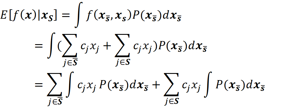
Suppose that there are k features in the set S̅. Since all these features are independent, we have:

By replacing this equation in the previous one, we have:

Since all the probabilities are normalized, we can write:
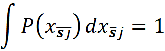
In addition, we have:
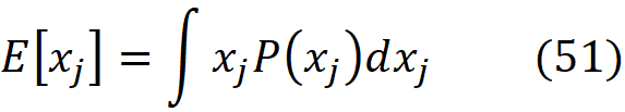
So, we have:
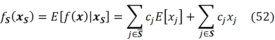
Now to calculate f_S∪{i}(x_S∪{i}) from fₛ(xₛ), we need to take the feature i from S̅ in Equation 52 and add it to S:
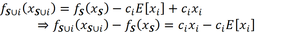
By replacing this equation in Equation 11 and using Equation 4, we get:
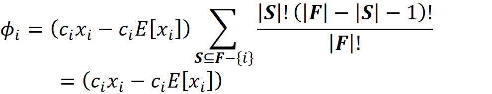
Please note that in Equation 51, we can only rely on a sample of the training data set to calculate the mean, so we have:
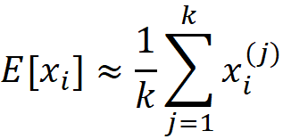
Here E[xᵢ] is the mean of xᵢ over all the instances of the sample of the training data set (k instances), and we have:
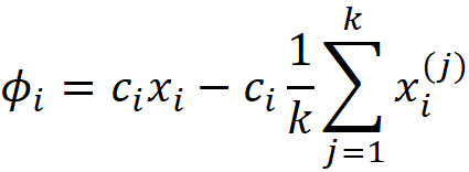
Proof of kernel SHAP theorem (theorem 1)
We assume that we have a feature vector x with M features. We first prove this for a case in which there are no missing features, so we have:

Then we calculate all the perturbations of x’. Each perturbation of x’ is a coalition vector with M elements, and each element can be either 0 or 1. So we have 2ᴹ perturbations. We call each perturbation z’ᵢ (which is a row vector). We place all these perturbations (or coalition vectors) in the 2ᴹ× M coalition matrix X:

For each coalition vector z’ᵢ , we can calculate the model prediction fₓ(zᵢ). We define the column vector y as:

where c₀ is a constant. In the original paper that introduced SHAP [1], c₀ is not included in y which is incorrect. We assume that
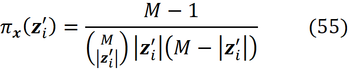
And we define the 2ᴹ× 2ᴹ diagonal matrix W as:
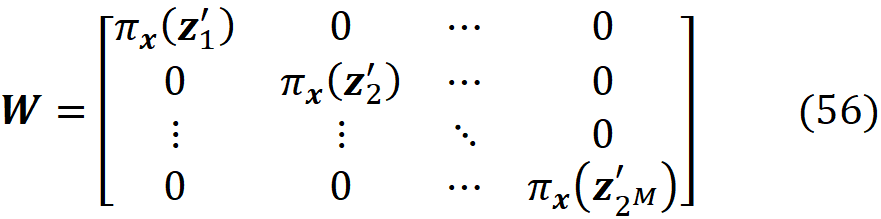
Now assuming that
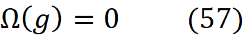
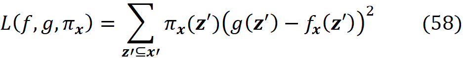
We need to show that as M goes to infinity the solution of
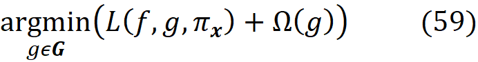
is
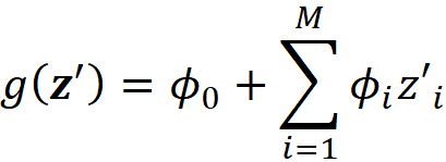
where ϕᵢ are the Shapley values of f and x defined in Equation 18. By replacing Equation 57 and Equation 58 in Equation 59 we get:
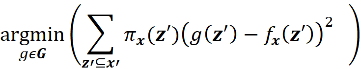
So, the objective function to be minimized is:

We can replace the coalition vectors z’ᵢ into Equation 60 to have:
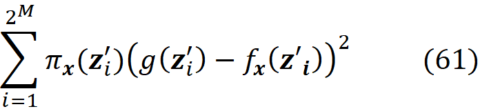
We limit our search for the optimal function g to linear functions with this form:
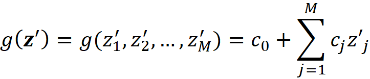
Here c₀ is the same constant used in Equation 54. For each coalition vector zᵢ, this equation is written as:

where [z’ᵢ]ⱼ is the j-th element of the coalition vector z’ᵢ. By replacing this equation in Equation 61 we have:
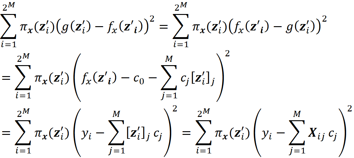
Here we used the fact that [z’ᵢ]ⱼ is the ij element of the matrix X in Equation 53 and yᵢ is the i-th element of the vector y in Equation 54. Now we define the column vector c as:
So, we can use the definition of matrix multiplication to write:
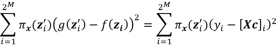
Please note that Xc is a column vector, and [Xc]ᵢ is its i-th element. We also know that πₓ(z’ᵢ) is the i-th diagonal element of the matrix W (Equation 56). So, we can again use the definition of matrix multiplication to write:
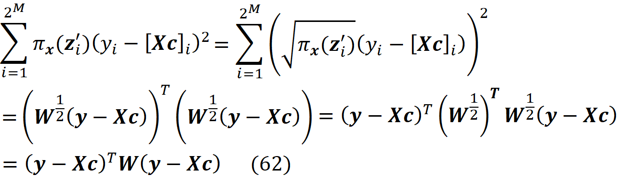
As a result, we conclude that:

Here we use the fact that g is only a function of cᵢ, so instead of finding the function g that minimizes the objective function, we find the value of the vector c that minimizes it. In fact, this objective function is similar to the loss function of a weighted linear regression model. Now we can minimize this objective function:
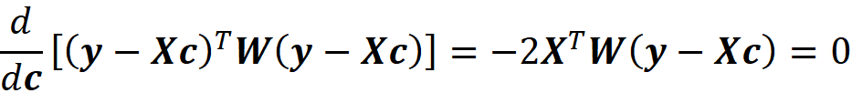
So, the value of c that minimizes the objective function is:

Now we need to simplify this equation. First, we simplify XᵀW:
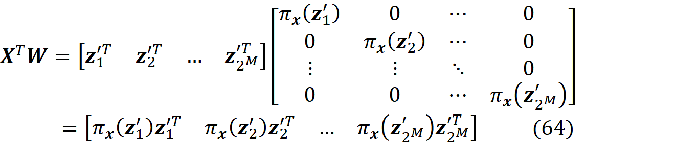
So, we have:
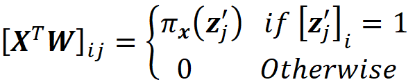
From Equation 64 we can conclude that the i-th row of XᵀW is:

And the j-th column of X is:
Now based on the definition of matrix multiplication, the ij element of XᵀWX is equal to the dot product of the i-th row of XᵀW and the j-th column of X:
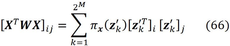
Now let’s look at the definition of πₓ(z’ᵢ):
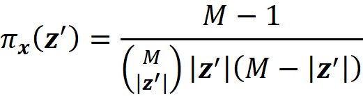
As you see it is a function of M and the number of non-zero entries in z’ (|z’|). So, for the same x:

In addition, we know that the maximum value of |z’ᵢ| is M. In Equation 66, if i=j, then we have:

Since z’ᵢ is a binary vector, [z’ₖ]ᵢ is either zero or one. So, we only need to include the terms for which [z’ₖ]ᵢ=1. Now in this equation, we can group all the summands for which |z’ᵢ| is a certain number say m. For each group πₓ(z’ᵢ) is the same (only a function of m):
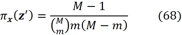
It is important to note that for m=0 (when all the elements of z’ᵢ are zero) and m=M (when all the elements of z’ᵢ are one), πₓ(z’ᵢ)=∞. However, it doesn’t affect this proof. For each value of m, we count the number of terms for which |z’ᵢ|=m and [z’ₖ]ᵢ=1, and we denote this count as:
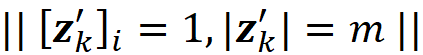
All these terms have the same πₓ(z’ᵢ). So, Equation 67 can be written as:
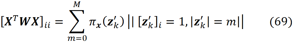
Similar, if i≠j, we have:
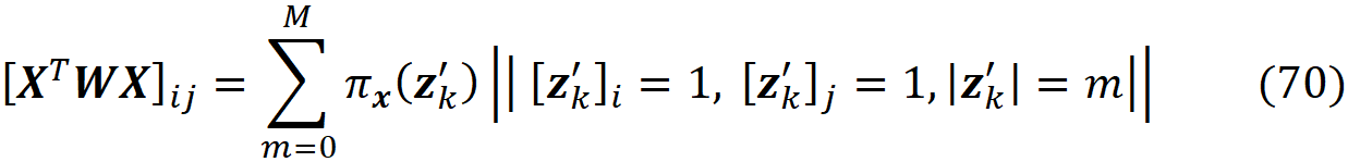
Now we need to calculate the value of
We know that the coalition vector z’ₖ has M elements. We want the i-th element to be 1. And the total number of 1s in z’ₖ should be m. So apart from the i-th element, we need m-1 elements of z’ₖ to be 1 and the rest to be 0. So, it is like choosing m-1 elements from the M-1 elements. So:
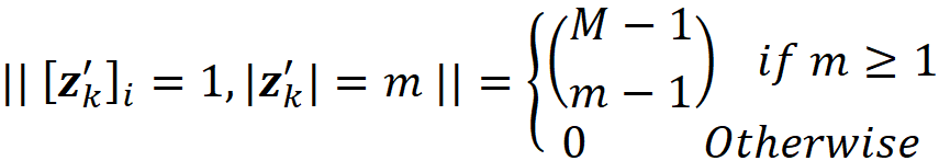
Similarly, we have:

By combining these equations with Equation 68, Equation 69, and Equation 70 we get:
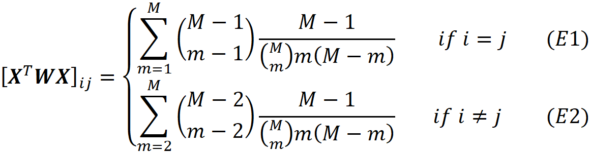
Based on this result all the diagonal elements of XᵀWX are equal to E1, and all the non-diagonal elements are equal to E2. So, we can write XᵀWX as:
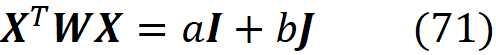
where I is the M×M identity matrix, and J is an M×M matrix of ones in which every element is equal to one. Now we need to calculate a and b in this equation. For non-diagonal elements of XᵀWX we have:

And for diagonal elements:

So, we have a system of two equations and by solving them we get:
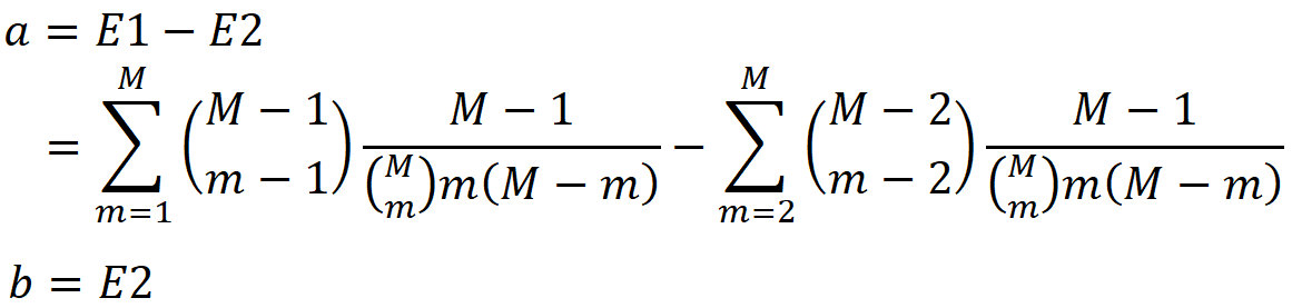
For m=M, the last two terms on the right-hand side of this equation cancel each other (though they both go to infinity):
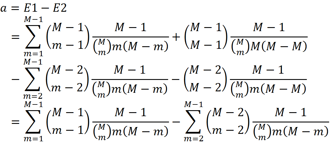
We can now simplify this equation:
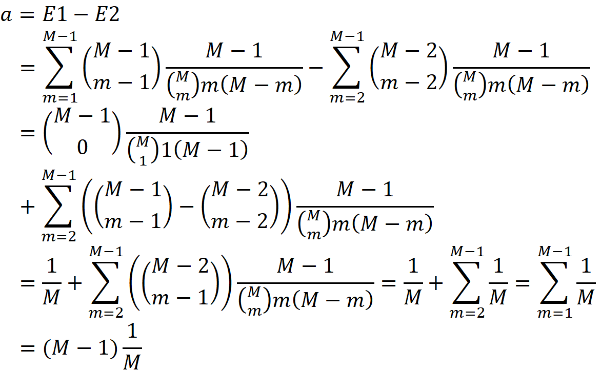
By inserting this equation into Equation 71 we have:
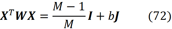
Now we want to calculate (XᵀWX)⁻¹. We can show that:
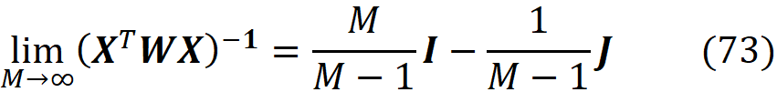
To prove that we should remember that for any matrix A:
Now we have:

For any M×M matrix like J we can easily show that:
By replacing this equation in the previous one we get:

So as M goes to infinity, the right-hand side of this equation becomes I. Similarly, we can show that:
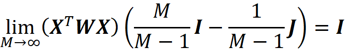
In the original paper that introduced SHAP [2], XᵀWX is not derived properly, however (XᵀWX)⁻¹ was still correct!
Now we need to calculate (XᵀWX)⁻¹XᵀW. From Equation 65 we know that the j-th column of XᵀW is πₓ(z’ⱼ)z’ⱼᵀ. The ij element of (XᵀWX)⁻¹XᵀW is the inner product of the i-th row of (XᵀWX)⁻¹ and the j-th column of XᵀW. From Equation 73, we know that
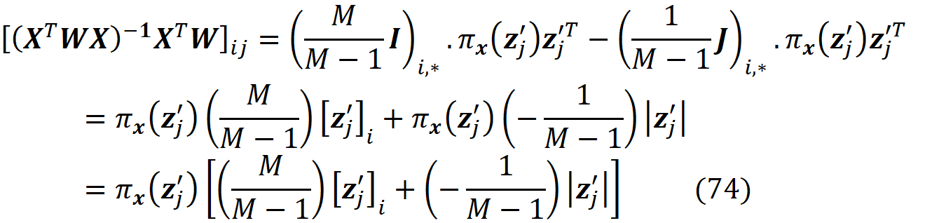
Where the subscript i,* denotes the i-th row of a matrix. Finally, we can calculate the vector c from Equation 63. The j-th element of the vector c is the inner product of the j-th row of the matrix (XᵀWX)⁻¹XᵀW and the i-th element of the vector y:
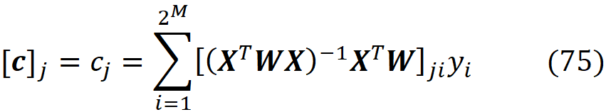
We first consider a coalition vector z’ᵢ for which [z’ᵢ]ⱼ=0. For such a vector we can use Equation 55 and Equation 74 and write:
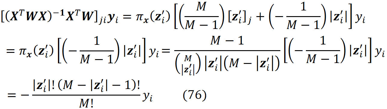
Then we consider a coalition vector z’ᵢ₊ which is equal to z’ᵢ with the j-th element set to 1. So, we can write:

We also assume that:
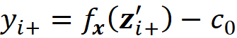
Now we can use Equation 74 and Equation 77 to write:
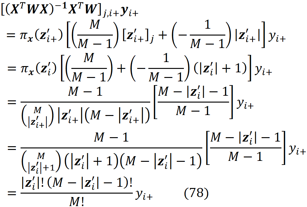
Combining Equation 76 and Equation 78 we have:
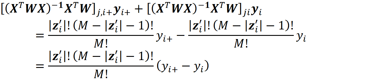
Finally, we can use Equation 75 to write:
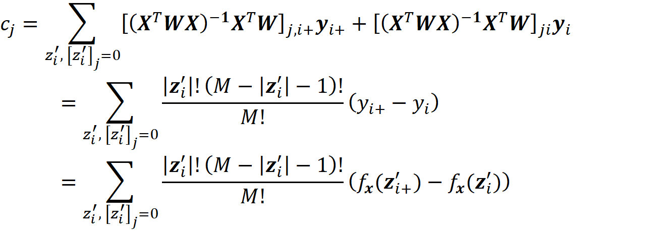
Instead of summing over z’ᵢ for which [z’ᵢ]ⱼ=0, we can sum over z’ᵢ₊. In that case, using Equation 77 we have:

Remember that for z’ᵢ₊ the j-th element is set to 1. However, we can also add any z’ᵢ in which [z’ᵢ]ⱼ=0. That’s because for such a coalition vector, fₓ(z’ᵢ₊)-fₓ(z’ᵢ)=0, so it doesn’t add anything to this sum, so we can add any coalition vector of x’ to this sum:
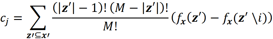
If we compare this equation with Equation 18 we conclude that:
So, the vector c gives the Shapley values of f and x, and the function that minimizes the objective function in Equation 61 has this form:
Which can be generally written as:
As you see, the minimization doesn’t determine the value of c₀. (It is like minimizing a function like y=x²+c where the minimum point is at x=0 no matter what the value of c is). To determine c₀, we set all the features to be NA, then z’ᵢ=0 for i=1..M. Hence, we have:
We also know that in that case, the model prediction is the average of the predictions of the instances in a sample of the training data set (Equation 22). So:

Hence, as M goes to infinity, we have:
where ϕ₀ =E[f(x)] and ϕᵢ (for i=1..M) give the Shapley values of f and x. For this proof, we initially assumed that |x’|=M, so x’ doesn’t have any zero elements, and x has no missing features. If we have some zero elements in x’ (|x’|< M), we only include the elements of x’ which are 1 (x’ᵢ=1) and the same proof applies to them. For the zero elements of x’ (which correspond to the missing features in x), we assume that ϕᵢ =0, and this is consistent with Equation 18.
Simplified equation of kernel SHAP solution
Consider the coalition matrix X defined in Equation 35 and let z’₁ and z’_2ᴹ be the all-zeros and all-ones coalitions respectively. We first create a new matrix called Xₜ by eliminating z’₁ and z’_2ᴹ from the coalition matrix X:
If we eliminate the terms corresponding to z’₁ and z’_2ᴹ in the objective function of Equation 40, we get:
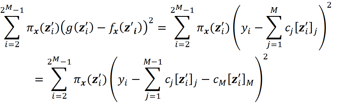
Now we can use Equation 43 to get:
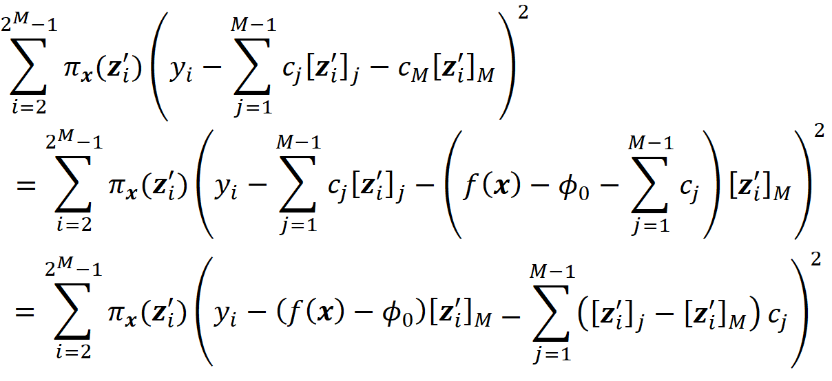
Please note that [z’ᵢ]_M is the M-th column of the matrix Xₜ. Now we can define the (2ᴹ-2)×(M-1) matrix Xᵣ as:
Here [Xₜ]_*,i is the i-th column of Xt. So Xᵣ is formed by subtracting the last column of Xₜ from the first M-1 columns. Now you can easily show that ij element of Xₜ is:
We also define the column vector cᵣ as:
and define the column vector yᵣ with 2ᴹ-2 elements as:
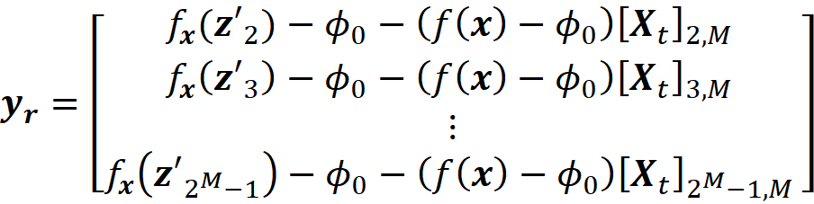
So, the i-th column of yᵣ is:
Now using the definition of matrix multiplication, we have:
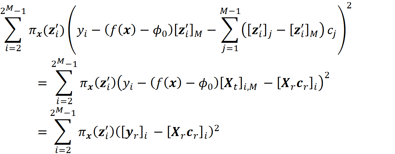
Finally, we define the (2ᴹ-2)× (2ᴹ-2) diagonal matrix Wᵣ as:
Now if we follow the same procedure that was used to simplify Equation 62 we get:
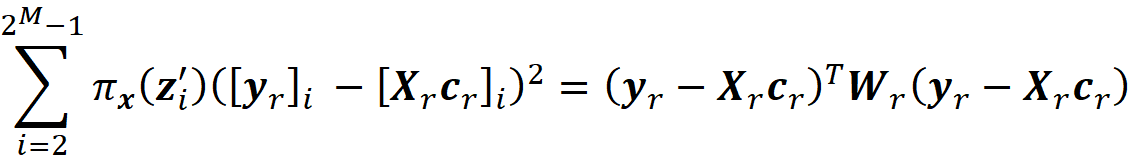
So, we need to solve this minimization problem:
and similar to Equation 63, the value of cᵣ that minimizes this objective function is:
No comments:
Post a Comment